Expected Shannon Diversity

We have a community that we’re describing with Shannon diversity, \(-\sum{p_ilogp_i}\) , but we’re doing so for a lot of sub-communities of different size. These diversities change with size in a way that is clearly not what we’d expect if they were simply samples from the regional pool, but to show that we need to see that expectation.

We should be able to get an analytical expected value given a set of regional proportions \(p_i…p_k\) and size of the sub-community \(N\). Most likely as a transformation of a multinomial distribution. But we’re under a bit of a time crunch, so I’ll throw together a bootstrap version.

Fundamentally, the null expectation for a sub-community of size \(N\) is defined as the identity of each individual being chosen from a categorical distribution with regional probabilities (pooled over all sub-communities) \(p_1…p_k\) , where \(k\) is the number of species. We could construct this with the Bernouilli, but the {extraDistr} package just has a random number generator.

extraDistr::rcat(10, c(0.1, 0.2, 0.3, 0.4))

 [1] 2 4 4 4 4 4 1 3 3 3

So, to bootstrap the expected shannon, for each n, we will do an rcat some large number of times, calculate shannon. That will give the probability distribution of the shannon, and the mean will be approximately the expectation. We might want other moments too, as sd should shrink as \(N\) increases.

expected_shannon <- function(N, regional_probs, 
                             n_boots = 1000, returntype = 'mean') {
  
  H <- matrix(NA, ncol = length(N), nrow = n_boots)
  colnames(H) <- paste0('N_', as.character(N))
  
  for (i in 1:length(N)) {
    for (j in 1:n_boots) {
      # This loses the names, but that doesn't matter.
      localcomp <- extraDistr::rcat(N[i], regional_probs)
      localprops <- table(localcomp)/N[i]
      H[j,i] <- -sum(localprops*log(localprops))
    }
  }
  
  if (returntype == 'dist') {return(H)}
  
  if (returntype == 'mean') {return(apply(H, 2, mean))}
  
}

A quick test

pooled_probs <- c(0.1, 0.5, 0.1, 0.3)
Es <- expected_shannon(1:100, regional_probs = pooled_probs)

plot(Es)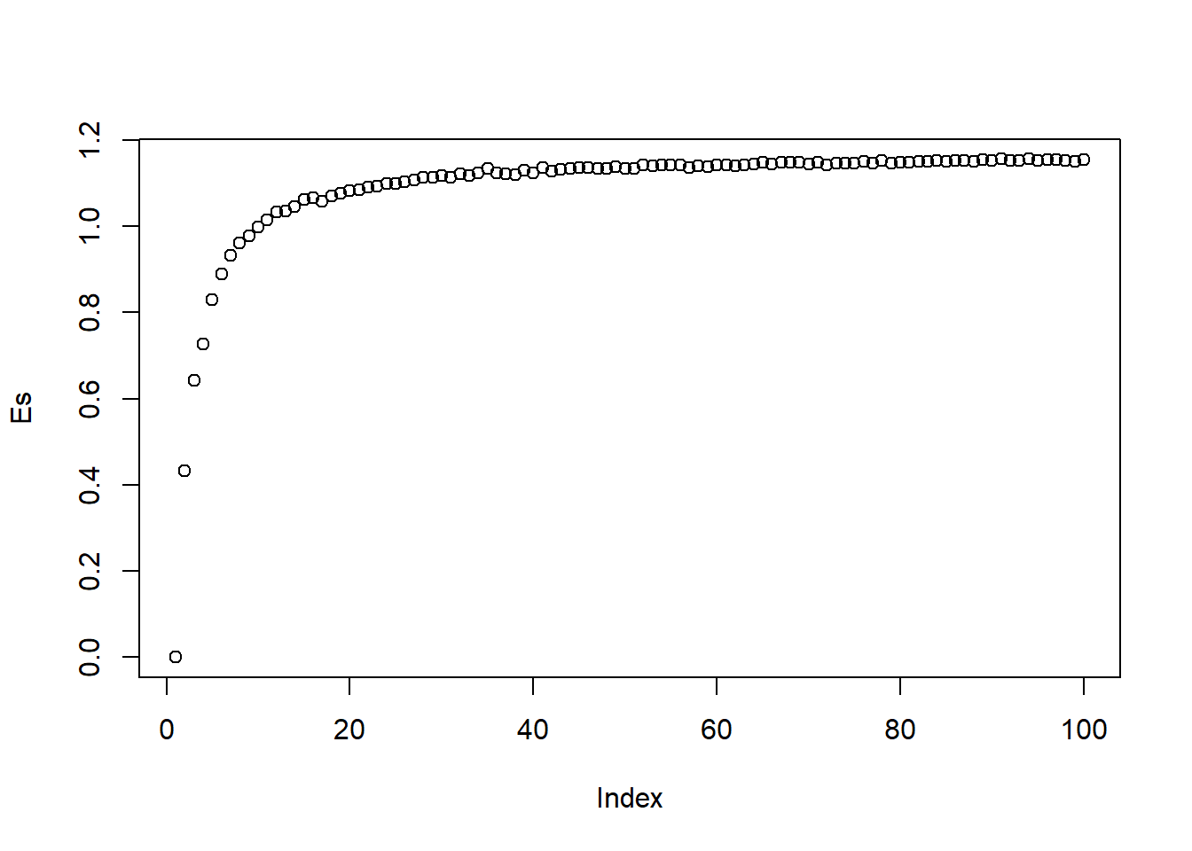

Larger N makes that take much larger, so we might want to do something like

Eslong <- expected_shannon(c(1:50, 100, 250, 500), 
                           regional_probs = pooled_probs)

plot(Eslong, type = 'lines')

Warning in plot.xy(xy, type, ...): plot type 'lines' will be truncated to first
character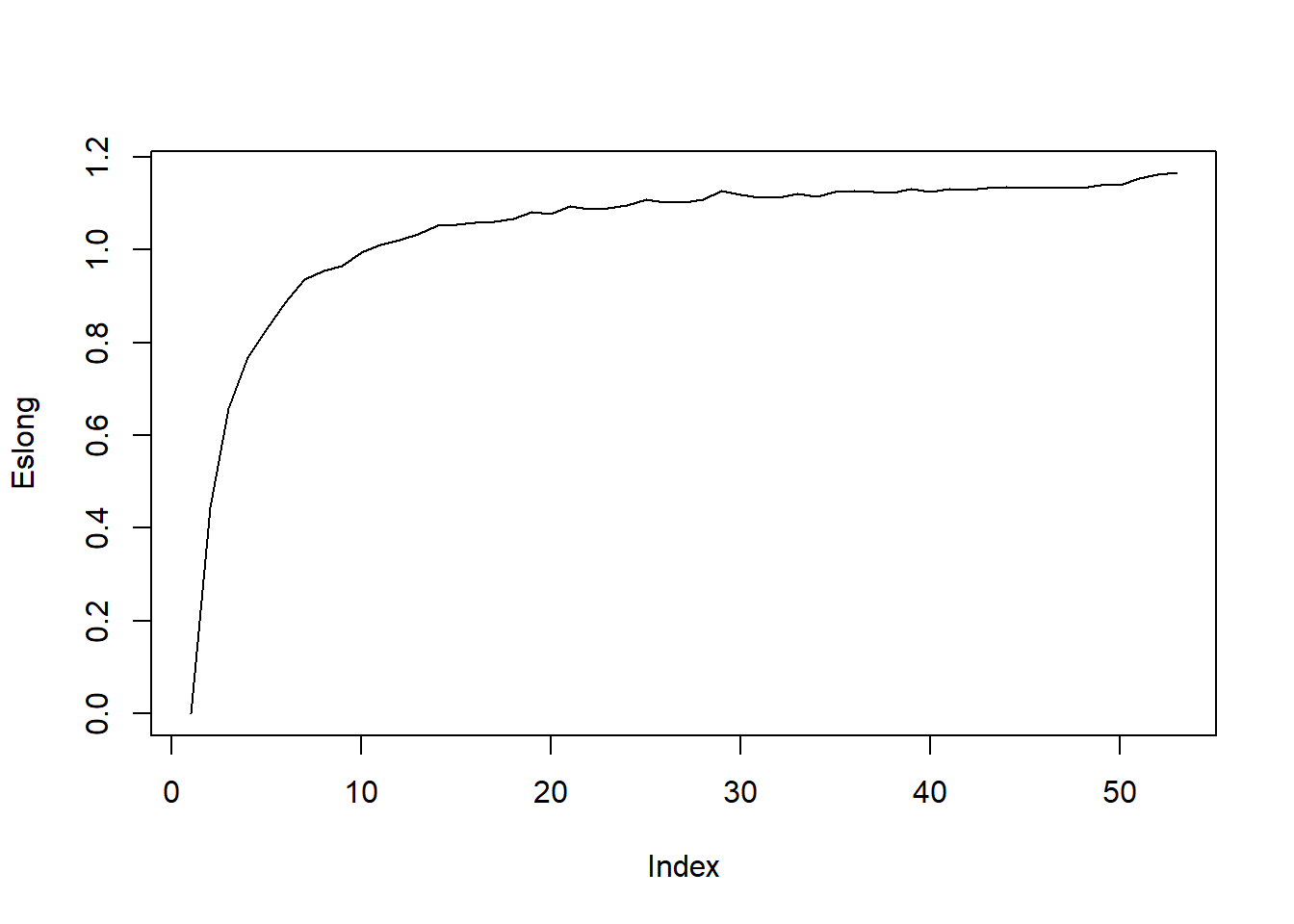

Simple- max and min

For reference, the max and min diversity occur at even p’s and only one p, respectively.

maxmin_shannon <- function(sp_range) {
  
  sp <- 1:sp_range
  
  maxshan <- rep(0, sp_range)
  minshan <- maxshan
  for (i in 1:sp_range) {
    minsp <- rep(0, i)
    minsp[1] <- 1
    maxsp <- rep(1/i, i)
    
    maxshan[i] <- -sum(maxsp*log(maxsp))
    minshan[i] <- -sum(minsp*log(minsp))
  }
  
  return(tibble::lst(minshan, maxshan))
  
}

The min is always 0, but the max depends nonlinearly on n species.

mms <- maxmin_shannon(100)

plot(mms$maxshan)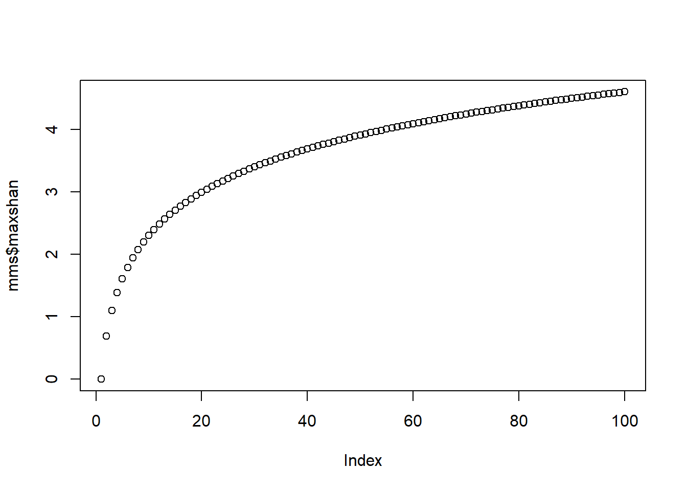

Analytically, for \(N\) species, the maximum shannon diversity is \[-N(1/N\ln{1/N})\], which collapses to \(\ln(N)\).