Rayshading

I want to figure out how to use rayshader. It has the potential to be really good for heatmaps, maps, etc.

library(tidyverse)

── Attaching core tidyverse packages ──────────────────────── tidyverse 2.0.0 ──
✔ dplyr     1.1.4     ✔ readr     2.1.5
✔ forcats   1.0.0     ✔ stringr   1.5.1
✔ ggplot2   3.5.1     ✔ tibble    3.2.1
✔ lubridate 1.9.3     ✔ tidyr     1.3.1
✔ purrr     1.0.2     
── Conflicts ────────────────────────────────────────── tidyverse_conflicts() ──
✖ dplyr::filter() masks stats::filter()
✖ dplyr::lag()    masks stats::lag()
ℹ Use the conflicted package (<http://conflicted.r-lib.org/>) to force all conflicts to become errors

library(rayshader)
library(sf)

Linking to GEOS 3.12.1, GDAL 3.8.4, PROJ 9.3.1; sf_use_s2() is TRUE

library(stars)

Loading required package: abind

Mostly I just want to play around with both making heatmaps and maps.

Plots

Let’s first see about using it to make 3d plots. The 2-d autocorr should be a good example. From that notebook, let’s generate some data.

# Load local functions
devtools::load_all()

ℹ Loading galenR

acmatrix_7_9 <- ac2d(n_x = 1000, n_y = 500,
        rho_x = 0.7, rho_y = 0.9,
        normVar = 1, printStats = TRUE)

[1] "Mean of all points is -0.012"
[1] "Var of all points is 1.006"
[1] "Mean y AC is 0.892"
[1] "Mean x AC is 0.698"

actib_7_9 <- tibble::as_tibble(acmatrix_7_9)  |> 
  mutate(y = row_number())  |> 
  pivot_longer(cols = starts_with('V'))  |> 
  mutate(x = as.numeric(str_remove(name, 'V')))  |> 
  select(-name)

Warning: The `x` argument of `as_tibble.matrix()` must have unique column names if
`.name_repair` is omitted as of tibble 2.0.0.
ℹ Using compatibility `.name_repair`.

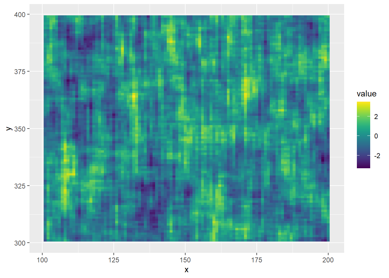
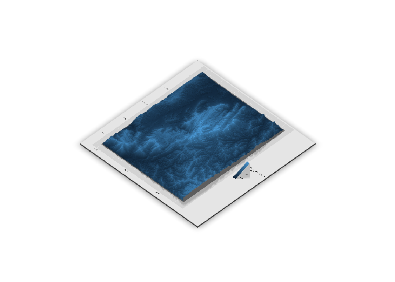
and the flat ggplot

gg2d <- ggplot(filter(actib_7_9, x > 100 & x <= 200 & y > 300 & y < 400), 
               aes(x = x, y = y, fill = value)) + 
  geom_tile() +
  viridis::scale_fill_viridis(option = 'viridis')

gg2d

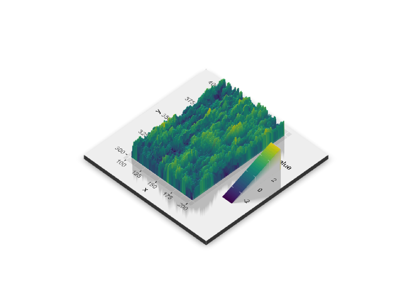
Rayshade version

There are a lot of arguments we can play with, but a simple default set works. Just have to remember to render_snapshot to see it.

plot_gg(gg2d)
render_snapshot(clear = TRUE)

A few tweaks, but basically, that’s what we want- the tweaks needed for any particular plot will be plot-specific.

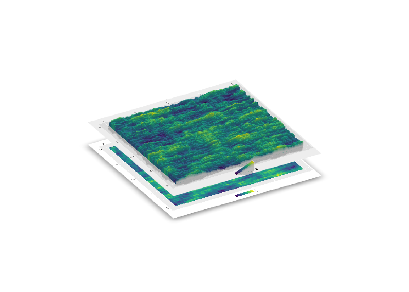
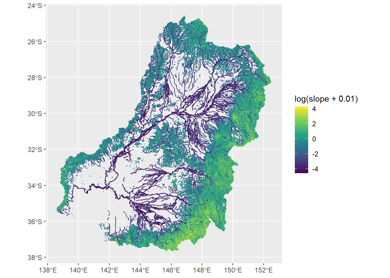
The flat_plot_render option is interesing, as it builds the typical heatmap as comparison.

plot_gg(gg2d, width = 10, height = 10, flat_plot_render = TRUE,
        # These are arguments passed to plot_3d, just playing around
        solid = FALSE,
        theta = 60,
        phi = 30)
render_snapshot()

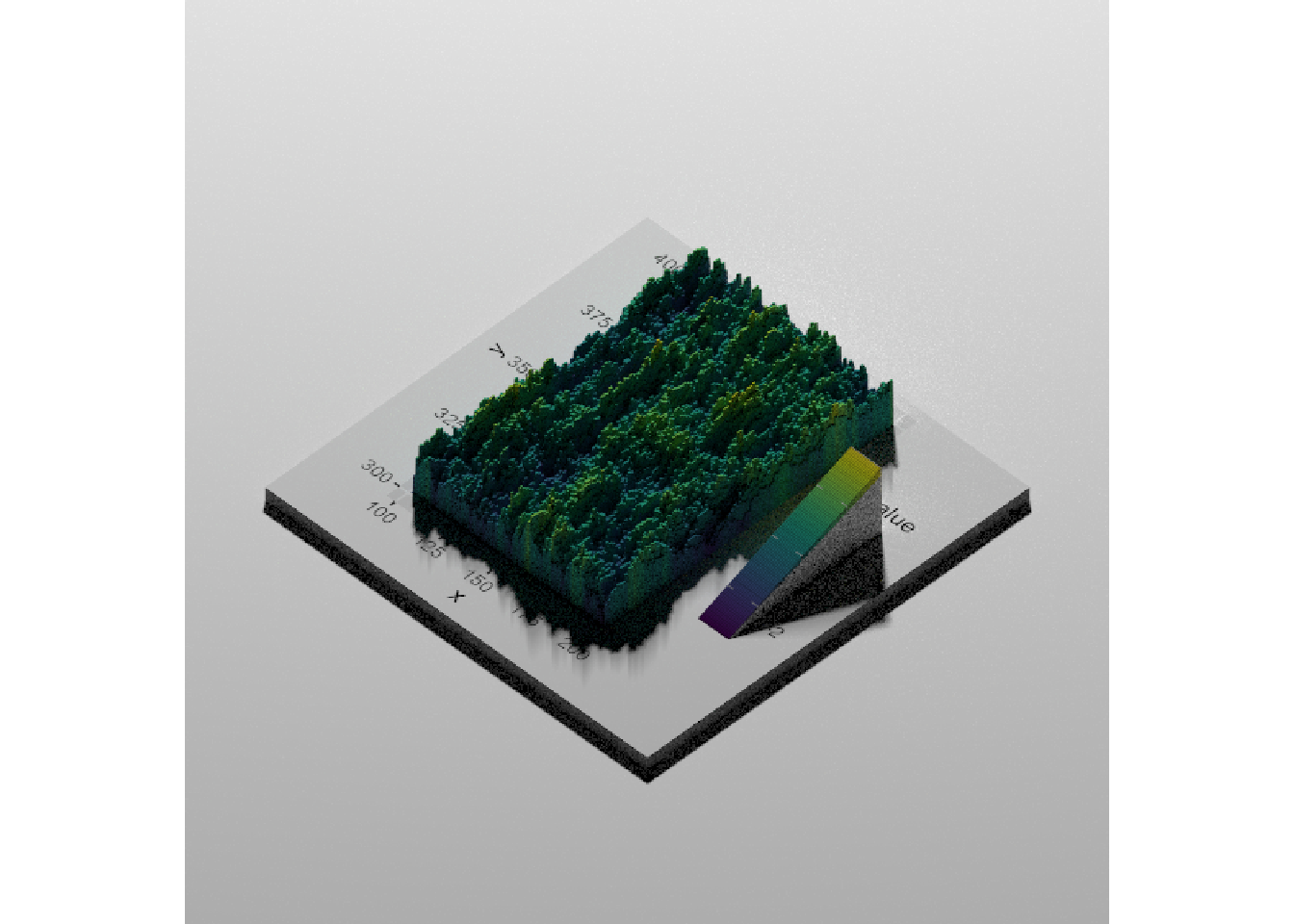
There’s also a render_highquality too, Though that seems to need some tweaks to look right, both in the notebook or the Rstudio viewer.

plot_gg(gg2d)
render_highquality(clear = TRUE)

Maps

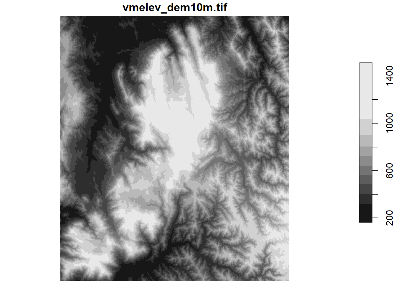
I found some huge DEMs, but figure I should start smaller, so I chose a small area of the 10m Vic DEM.

I’d typically use stars, but the examples all use raster. Not sure it’ll work with stars.

vicdem <- read_stars(file.path('data', 'DATA_362071', 'VIC Government', 'DEM', '10 Metre', 'vmelev_dem10m.tif'))

Plot that with plot.stars

plot(vicdem)

downsample set to 3

Now, can I make a map? The examples use raster, but I think we need a matrix. Each sheet in the stars is a matrix, so just get it directly.

vicdem[[1]] %>%
  sphere_shade(texture = "imhof2") %>%
  plot_map()

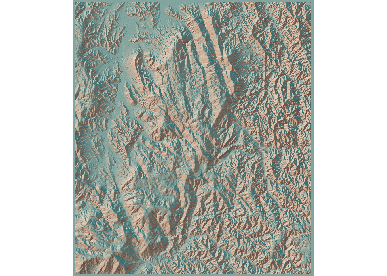
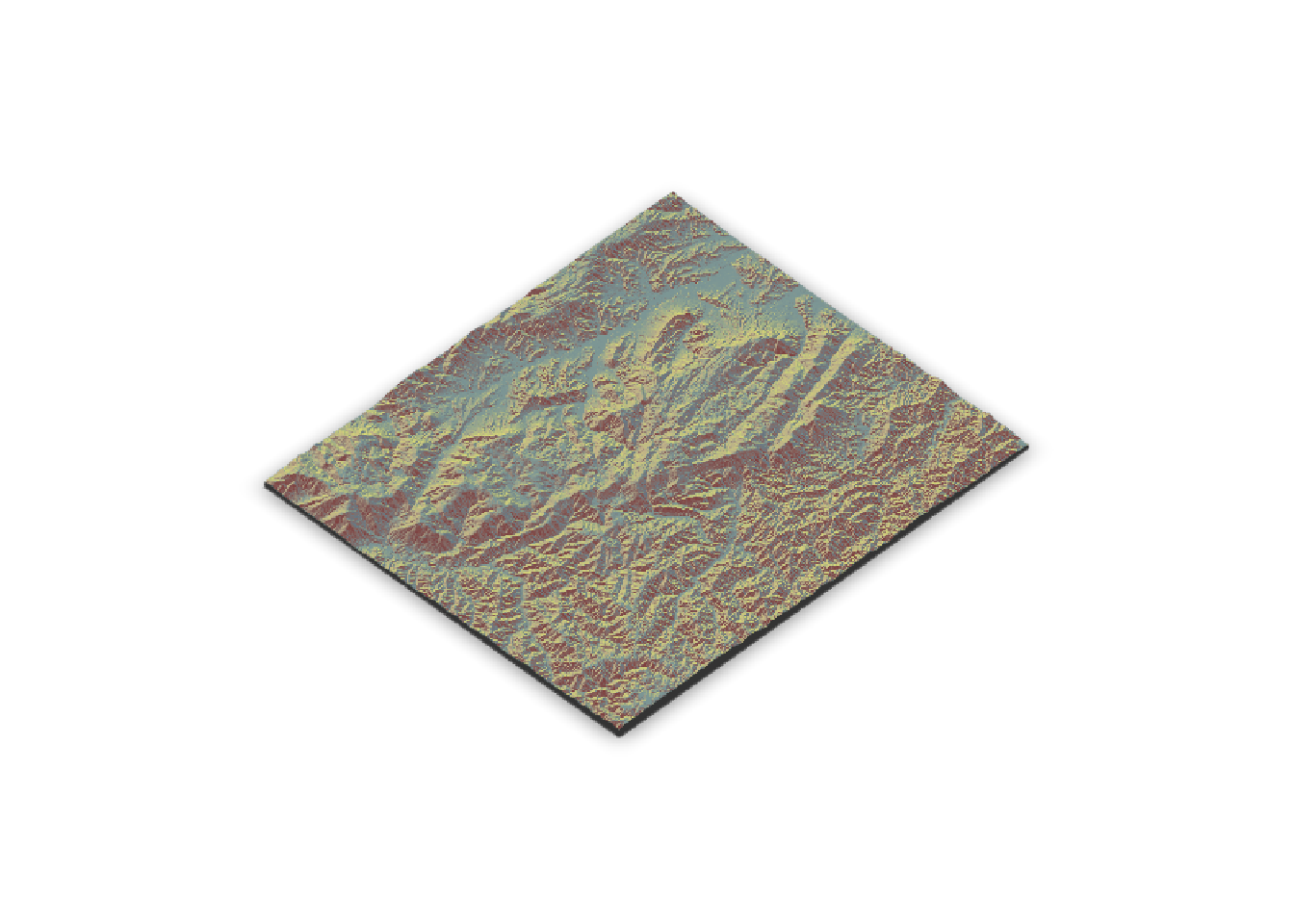
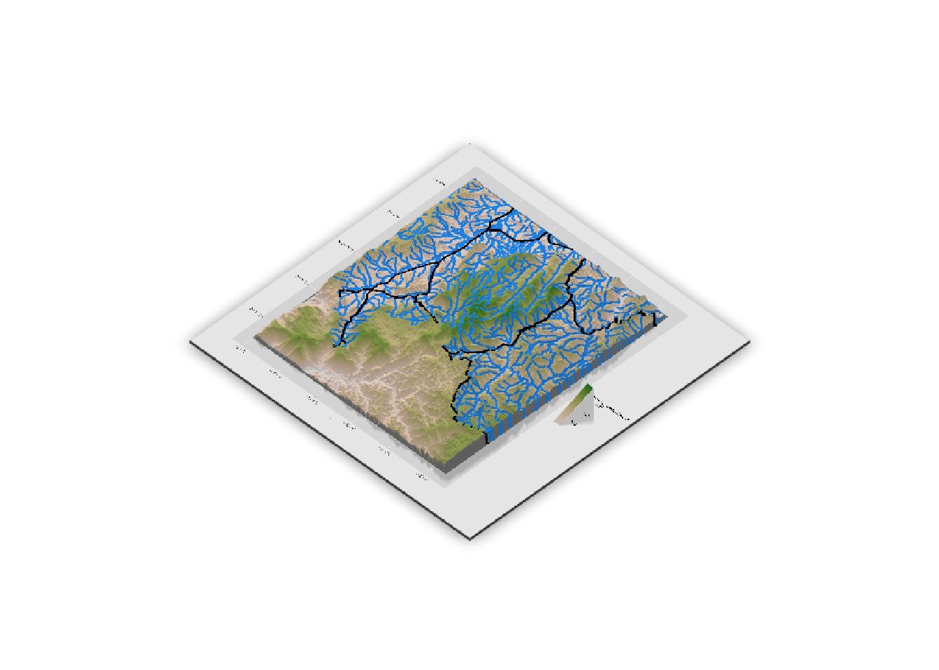
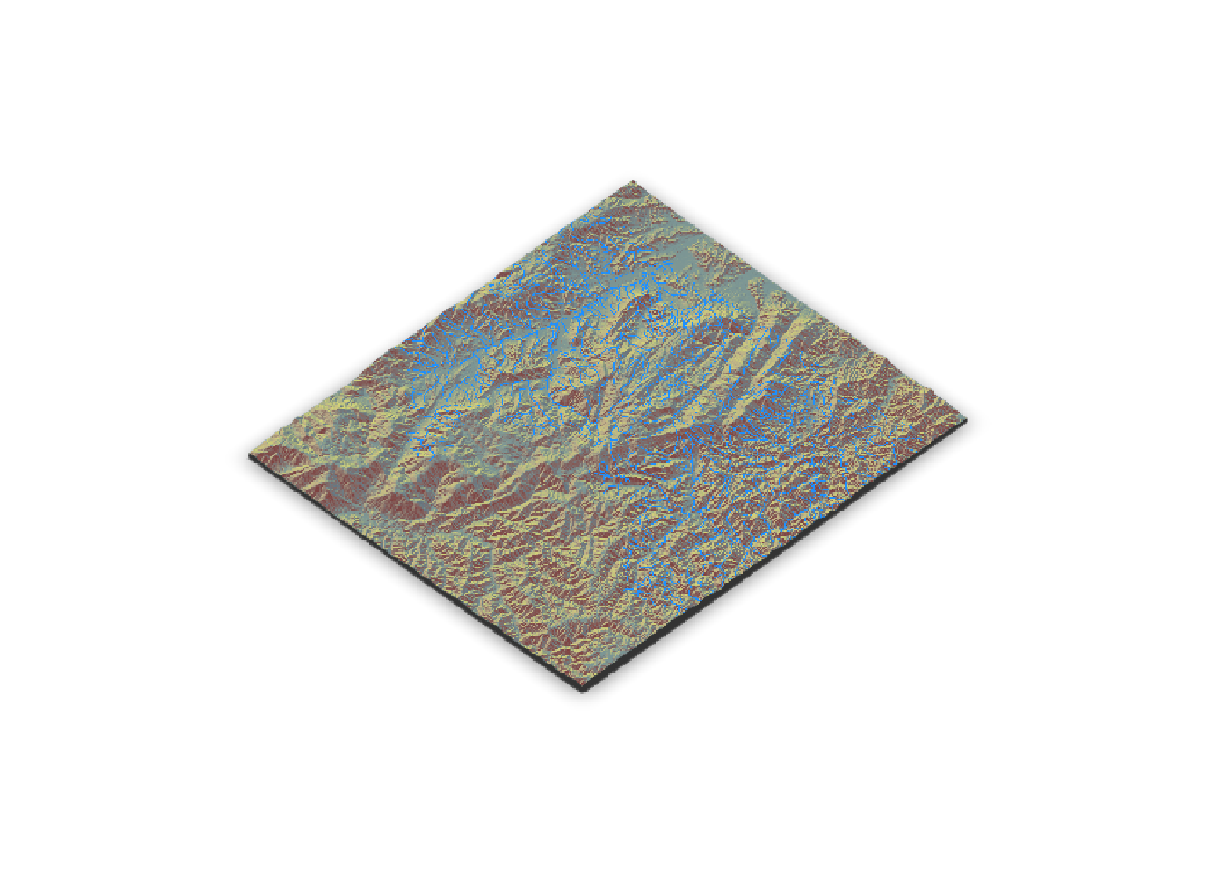
Make it 3d- this is interesting. It takes the DEM as the second argument too, because the arguments are hillshade, which is generated by sphere_shade and heightmap, which is just the DEM.

vicdem[[1]] %>%
  sphere_shade(texture = "imhof3") %>%
  plot_3d(vicdem[[1]], zscale = 10)

render_snapshot()

Can we use geom_stars to generate a {rayshader} fig from plot_gg?

demgg <- ggplot() +
  geom_stars(data = vicdem)
demgg

Try the plot_gg. It does have some hillshade- easier to confirm if we move it around in the window that pops up.

plot_gg(demgg, width = 10, height = 10)
render_snapshot()

Now I want to overlay stream lines and municipalities on there. Will need to get those shapefiles.

The BOM geofabric is in the ANAE, and I have that already. So

streams <- sf::read_sf(file.path('data', 'ANAE_Rivers_v3_23mar2021', 'ANAE_Rivers_v3_23mar2021', 'Waterways_ANAE_Geofabric3.shp'))

That makes a nice plot just on its own

streams |> 
  dplyr::mutate(slope = ifelse(slope < 0, 0, slope)) |> 
  ggplot() +
  geom_sf(mapping = aes(color = log(slope + 0.01))) +
  scale_color_viridis_c()

Get towns and roads- Marysville is about the only town in the chosen area of the victorian DEM?

towns <- sf::read_sf(dsn = file.path('data', 'MDB_ANAE_Aug2017/MDB_ANAE.gdb'), layer = 'MajorTowns')
roads <- sf::read_sf(dsn = file.path('data', 'MDB_ANAE_Aug2017/MDB_ANAE.gdb'), layer = 'MajorRoads')

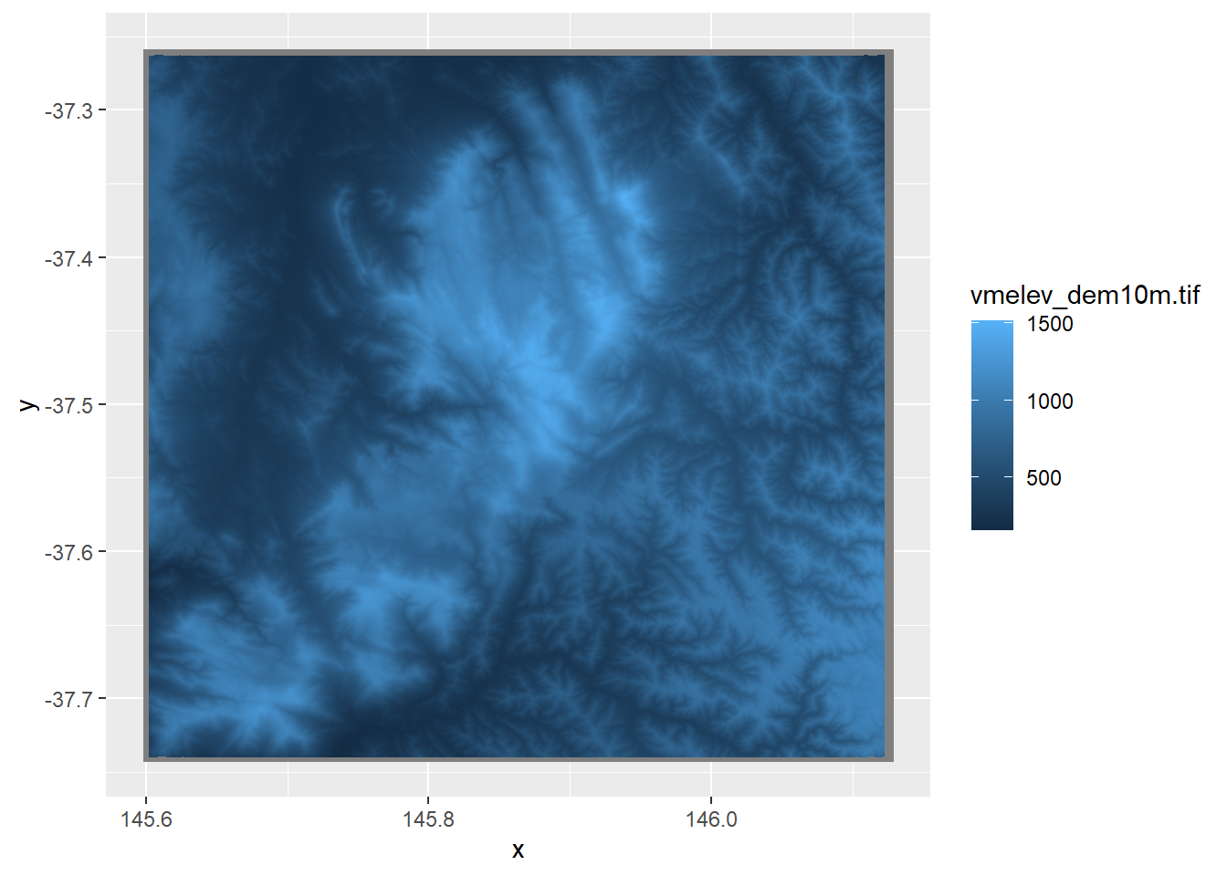
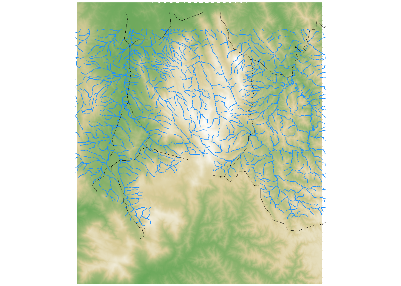
Clip to the vicdem. This is a bit funny, because the streams_mville dataset from the ANAE is clipped to the Murray-Darling Basin, but the DEM is only partially in the basin, and so we lose some of it.

vicbb <- st_bbox(vicdem) |> st_as_sfc()

streams_mville <- streams |> 
  st_transform(st_crs(vicdem)) |> 
  st_intersection(vicbb)

Warning: attribute variables are assumed to be spatially constant throughout
all geometries

towns <- towns |> 
  st_transform(st_crs(vicdem)) |> 
  st_intersection(vicbb)

Warning: attribute variables are assumed to be spatially constant throughout
all geometries

roads <- roads |> 
  st_transform(st_crs(vicdem)) |> 
  st_intersection(vicbb)

Warning: attribute variables are assumed to be spatially constant throughout
all geometries

Quick gg

demgg_streams_mville <- ggplot() +
  geom_stars(data = vicdem) +
  geom_sf(data = streams_mville, color = 'dodgerblue', linewidth = 2) +
  geom_sf(data = roads, color = 'black', linewidth = 2) +
  #geom_sf(data = towns, color = 'firebrick') +
  colorspace::scale_fill_continuous_sequential(palette = 'Terrain 2')
#demgg_streams_mville

Use plot_gg

plot_gg(demgg_streams_mville, width = 10, height = 10)
render_snapshot()

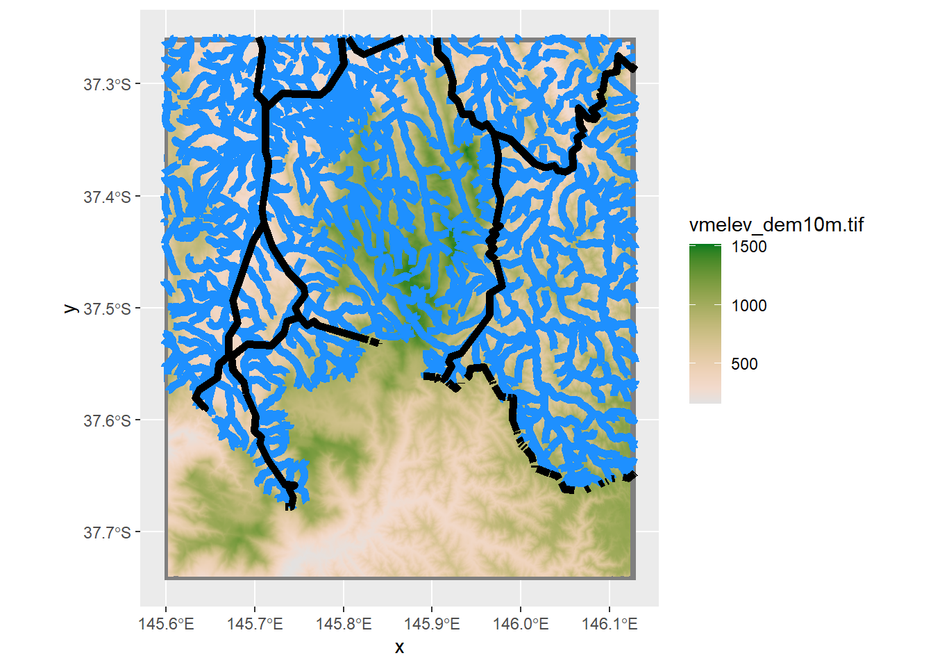
The streams don’t really show up well. Do they with a flat map? is it just that they’re too narrow to render well in 3d?

demgg_streams_mville

Can I make that with plot3d? I can’t get the extent argument to work without passing heightmap as well. Not sure why- they seem to both define the cropping extent.

Can I get it to work at all? Using almost exactly the example code, just modified for this dataset. Those are really wonky, and it’s not because of an issue with height- the roads were just given a length and width. I have to make the streams have huge linewidth to see them.

vicdem[[1]] |> 
  height_shade() |> 
  add_overlay(generate_line_overlay(streams_mville, color = 'dodgerblue',
                                    extent = st_bbox(vicdem),
                                    heightmap = vicdem[[1]],
                                    linewidth = 10)) |> 
  add_overlay(generate_line_overlay(roads, color = 'black',
                                     extent = st_bbox(vicdem),
                                    width = 1080, height = 1080)) |> 
  plot_map()

So does this not work because the streams_mville just get lost? e.g. are they there, they just don’t show up?

vicdem[[1]] %>%
  sphere_shade(texture = "imhof3") |> 
  # add_overlay(generate_line_overlay(roads, color = 'black',
  #                                   extent = attr(vicdem[[1]], 'extent'))) |> 
  # add_overlay(generate_point_overlay(towns, color = 'firebrick',
  #                                   extent = attr(vicdem[[1]], 'extent'))) |> 
    add_overlay(generate_line_overlay(streams_mville, color = 'dodgerblue',
                                    extent = st_bbox(vicdem),
                                    heightmap = vicdem[[1]],
                                    linewidth = 10)) |> 
  plot_3d(vicdem[[1]], zscale = 10)


render_snapshot()

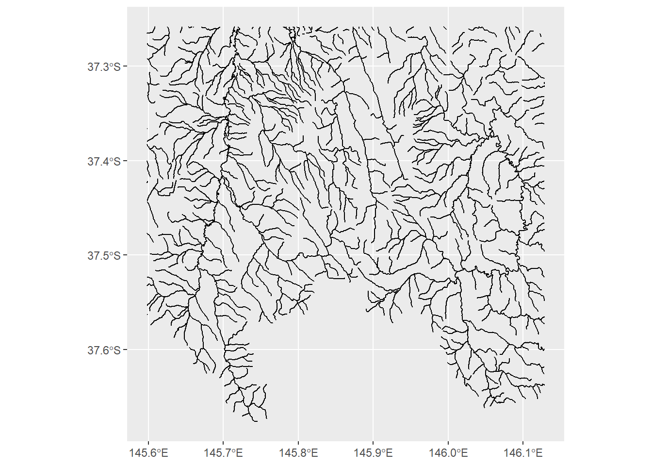
The streams layer itself isn’t so bad when looked at alone. So somehow it’s sort of disintegrating when used as an overlay, whether with the gg method or not.

ggplot(streams_mville) + geom_sf()