Read australia geofabric

library(sf)

Linking to GEOS 3.12.1, GDAL 3.8.4, PROJ 9.3.1; sf_use_s2() is TRUE

library(dplyr)

Attaching package: 'dplyr'

The following objects are masked from 'package:stats':

    filter, lag

The following objects are masked from 'package:base':

    intersect, setdiff, setequal, union

library(ggplot2)

We downloaded and saved the geofabric. Now we want to open and plot some of it.

The folder structure is too complex inside the zip, so have to extract. I’m most interested right now in the river lines.

gdbpath <- file.path('data', 'geofabric', 'SH_Network_GDB', 'SH_Network.gdb')
if (!file.exists(gdbpath))
  
unzip(file.path('data', 'geofabric', 'SH_Network_GDB_V3_3.zip'),
      exdir = file.path('data', 'geofabric'))

There are a lot of layers, so can’t just st_read

st_layers(gdbpath)

Driver: OpenFileGDB 
Available layers:
                    layer_name     geometry_type features fields crs_name
1    AHGFNetworkConnectivityUp                NA  3694332      3     <NA>
2  AHGFNetworkConnectivityDown                NA  2642087      3     <NA>
3         AHGFNetworkStream_FS                NA   120614      2     <NA>
4           AHGFNetworkNodeLUT                NA     6370     14     <NA>
5              AHGFNetworkNode             Point  2532980     29    GDA94
6                AHGFCatchment     Multi Polygon  7047524     27    GDA94
7            AHGFNetworkStream Multi Line String  2578471     31    GDA94
8                AHGFWaterbody     Multi Polygon   159198     27    GDA94
9     SH_Network_Net_Junctions             Point        0      1    GDA94
10                    N_1_Desc                NA  5117450      5     <NA>
11                   N_1_EDesc                NA     1893      2     <NA>
12                 N_1_EStatus                NA       40      2     <NA>
13                   N_1_ETopo                NA      631      2     <NA>
14                  N_1_FloDir                NA       40      2     <NA>
15                   N_1_JDesc                NA     1856      2     <NA>
16                 N_1_JStatus                NA       39      2     <NA>
17                   N_1_JTopo                NA     4948      2     <NA>
18                  N_1_JTopo2                NA        2      2     <NA>
19                   N_1_Props                NA        9      2     <NA>

The stream lines are big, but just reading doesn’t take too long.

rivers <- st_read(gdbpath, layer = 'AHGFNetworkStream')

Reading layer `AHGFNetworkStream' from data source 
  `C:\Users\galen\Documents\code\web_testing\galen_website\data\geofabric\SH_Network_GDB\SH_Network.gdb' 
  using driver `OpenFileGDB'
Simple feature collection with 2578471 features and 31 fields
Geometry type: MULTILINESTRING
Dimension:     XY
Bounding box:  xmin: 113.3753 ymin: -43.62889 xmax: 153.6317 ymax: -10.06028
Geodetic CRS:  GDA94

Let’s subset to the major rivers to not crash?

major_rivers <- rivers |> 
  dplyr::filter(Hierarchy == 'Major')

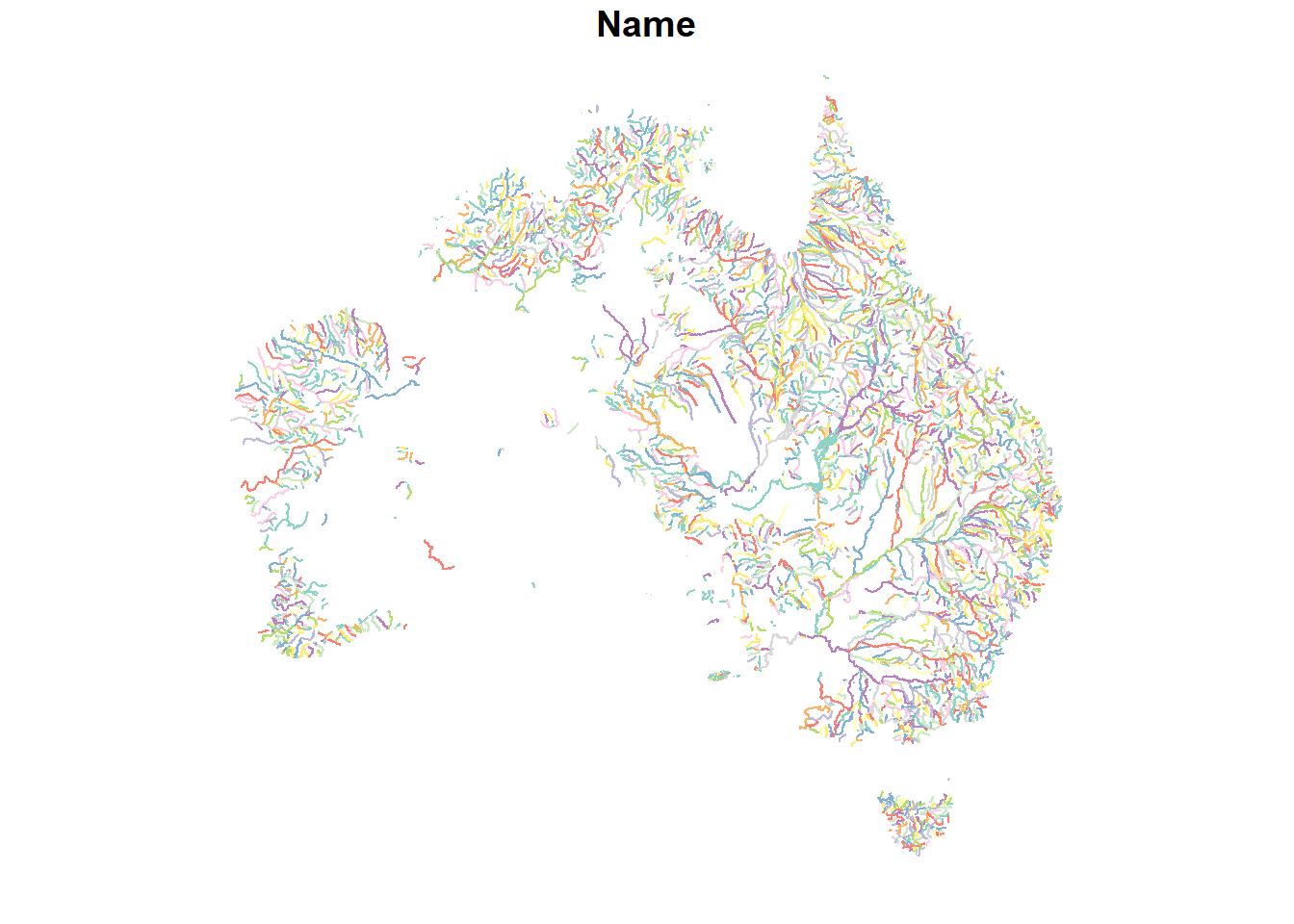
Still 182557, but we can try to plot it?

plot(major_rivers[,'Name'])

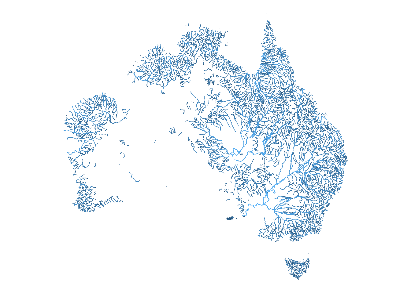
riverlen_plot <- ggplot(major_rivers, aes(color = log(UpstrGeoLn))) +
  geom_sf() +
  theme_void()

riverlen_plot + theme(legend.position = 'none')