Beta distributions

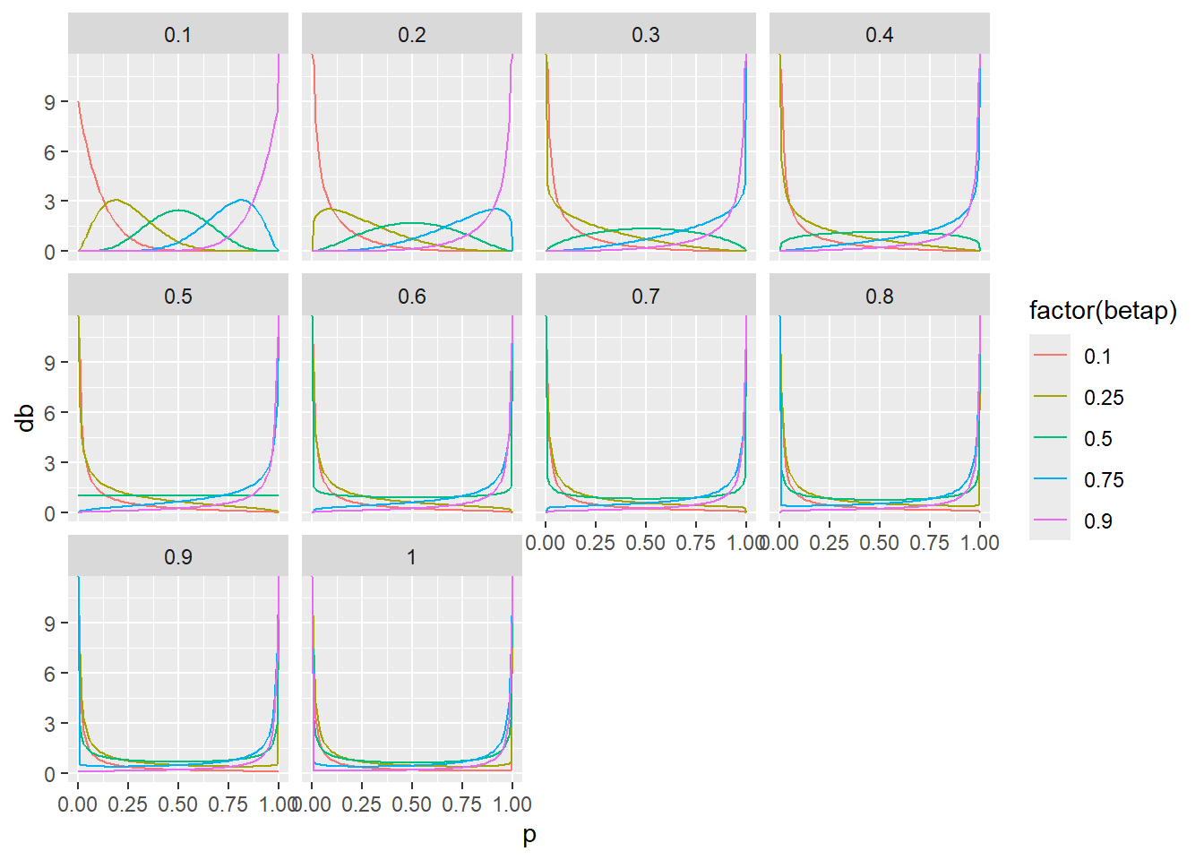
This is fairly sketchy, just trying to see how the \(\phi\) from Harrison (2015) affect beta probability distributions.

library(tidyverse)

── Attaching core tidyverse packages ──────────────────────── tidyverse 2.0.0 ──
✔ dplyr     1.1.4     ✔ readr     2.1.5
✔ forcats   1.0.0     ✔ stringr   1.5.1
✔ ggplot2   3.5.1     ✔ tibble    3.2.1
✔ lubridate 1.9.3     ✔ tidyr     1.3.1
✔ purrr     1.0.2     
── Conflicts ────────────────────────────────────────── tidyverse_conflicts() ──
✖ dplyr::filter() masks stats::filter()
✖ dplyr::lag()    masks stats::lag()
ℹ Use the conflicted package (<http://conflicted.r-lib.org/>) to force all conflicts to become errors

p <- seq(from = 0, to = 1, by = 0.01)
phi <- seq(from = 0.1, to = 1, by = 0.1)

# ai <- p[1]/phi[1]
# bi <- (1-p[1])/phi[1]
# 
# db <- dbeta(p, ai, bi)

probdists <- tibble(p = NA, db = NA, betap = NA, phi = NA, .rows = 0)

for (j in 1:length(phi)) {
  for (i in 1:length(p)) {
  ai <- p[i]/phi[j]
  bi <- (1-p[i])/phi[j]
  
  db <- dbeta(p, ai, bi)
  
  dbt <- tibble(p, db, betap = p[i], phi = phi[j])
  probdists <- rbind(probdists, dbt)
}
}

ggplot(probdists |> filter(betap %in% c(0.1, 0.25, 0.5, 0.75, 0.9)), 
       aes(x = p, y = db, color = factor(betap))) + geom_line() +
  facet_wrap("phi")

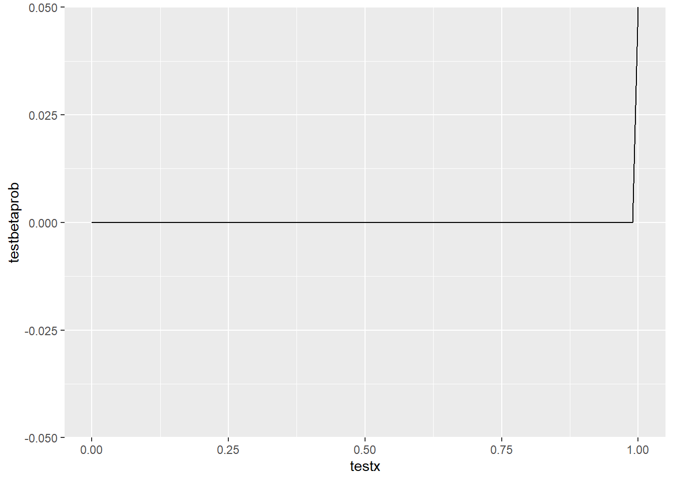
testx <- seq(from = 0, to = 1, by = 0.01)
testbetaprob <- dbeta(testx, ai, bi)
probdist <- tibble(testx, testbetaprob)

ggplot(probdist, aes(x = testx, y = testbetaprob)) + geom_line()

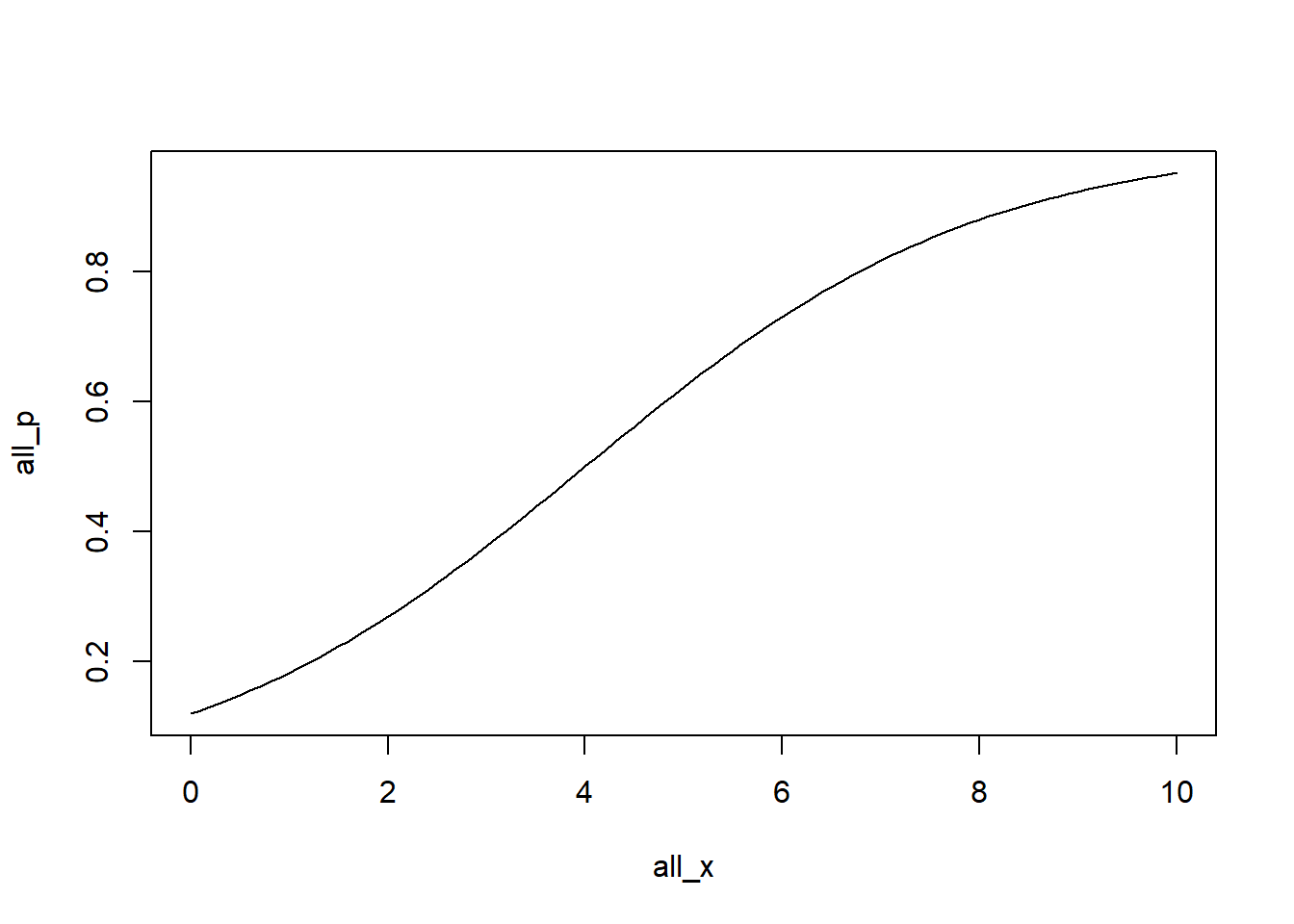
Random draws

intercept <- -2
beta <- 0.5
all_x <- seq(0, 10, 0.1)
all_logit_p <- intercept + beta*all_x

all_p <- 1/(1+exp(-all_logit_p))

plot(all_x, all_p, type = 'l')

References

Harrison, Xavier A. 2015. “A Comparison of Observation-Level Random Effect and Beta-Binomial Models for Modelling Overdispersion in Binomial Data in Ecology & Evolution.” PeerJ 3 (July): e1114. https://doi.org/10.7717/peerj.1114.