HydroSHEDS/RIVERS/ATLAS

library(sf)
library(ggplot2)
library(dplyr)
devtools::load_all()

ℹ Loading galenR

HydroSHEDS has BASINS, RIVERS, LAKES, and ATLAS, with the atlas being versions of the others with covariates.

I’m mostly interested in the rivers and sheds atlases. For now, get rivers.

ratlas <- "https://figshare.com/ndownloader/files/20087321"

zipdownload('RiverATLAS_Data_v10.gdb', 'data', ratlas)

[1] TRUE

What layers are in that gdb?

st_layers(file.path('data',
                    'RiverATLAS_Data_v10', 'RiverATLAS_v10.gdb'))

Driver: OpenFileGDB 
Available layers:
      layer_name     geometry_type features fields crs_name
1 RiverATLAS_v10 Multi Line String  8477883    296   WGS 84

Only one layer, but pretty big (it is the whole world), probably worth using the query argument.

The docs have a pdf of available columns. The real trick is going to be figuring out their values so we can filter on them.

Those are in HydroATLAS_v10_Legends.xlsx.

Can I get the available countries (global administrative areas)?

gad_ids <- st_read(file.path('data',
                    'RiverATLAS_Data_v10', 'RiverATLAS_v10.gdb'),
                   query = sprintf("SELECT DISTINCT gad_id_cmj FROM \"%s\"", 'RiverATLAS_v10'))

Reading query `SELECT DISTINCT gad_id_cmj FROM "RiverATLAS_v10"'
from data source `C:\Users\galen\Documents\code\web_testing\galen_website\data\RiverATLAS_Data_v10\RiverATLAS_v10.gdb' 
  using driver `OpenFileGDB'

Warning: no simple feature geometries present: returning a data.frame or tbl_df

Those aren’t particularly useful on their own. Are they ISO codes? Supposedly, but they don’t match the numerics.

That suggests Australia is 036, but HydroATLAS_v10_Legends.xlsx has it as 14. The country_code does match though.

This takes a LONG time, and only returns 5375 shapes, which is way fewer than HydroRIVERS has for Australia.

aus_rivers <- st_read(file.path('data',
                    'RiverATLAS_Data_v10', 'RiverATLAS_v10.gdb'),
                   query = sprintf("SELECT * FROM \"%s\" WHERE gad_id_cmj = 14", 'RiverATLAS_v10'))

Reading query `SELECT * FROM "RiverATLAS_v10" WHERE gad_id_cmj = 14'
from data source `C:\Users\galen\Documents\code\web_testing\galen_website\data\RiverATLAS_Data_v10\RiverATLAS_v10.gdb' 
  using driver `OpenFileGDB'
Simple feature collection with 359556 features and 296 fields
Geometry type: MULTILINESTRING
Dimension:     XY
Bounding box:  xmin: 112.9271 ymin: -54.73958 xmax: 158.9187 ymax: -9.23125
Geodetic CRS:  WGS 84

Mapping that

ggplot() +
  geom_sf(data = aus_rivers |> filter(ORD_STRA >= 3), mapping = aes(color = log10(DIST_UP_KM)))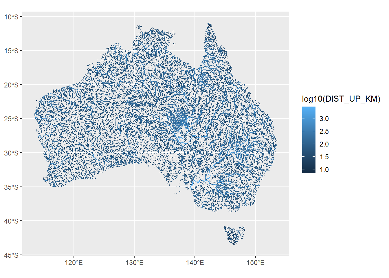

We can also use a spatial filter see wkt_filter argument to pass e.g. a bounding box. I’m guessing that’s super slow.

Some other interesting variables

irrigated area upstream

ggplot() +
  geom_sf(data = aus_rivers |> filter(ORD_STRA >= 3), mapping = aes(color = log10(ire_pc_use)))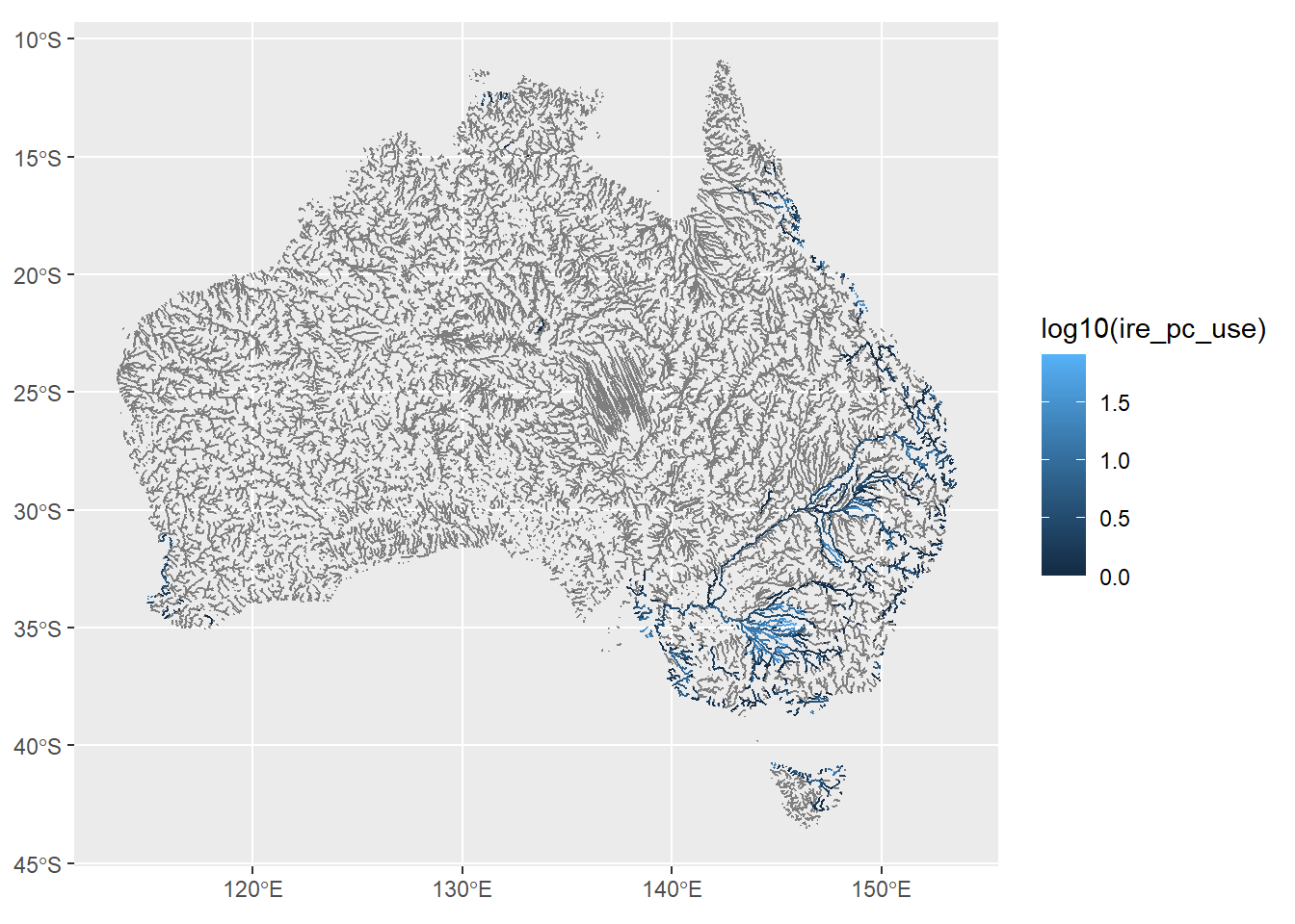

PET

ggplot() +
  geom_sf(data = aus_rivers |> filter(ORD_STRA >= 3), mapping = aes(color = (pet_mm_uyr))) +
  scale_color_viridis_c(option = 'inferno')

precip

ggplot() +
  geom_sf(data = aus_rivers |> filter(ORD_STRA >= 3), mapping = aes(color = pre_mm_uyr)) +
  scale_color_viridis_c(option = 'mako', trans = 'log10')

temp

ggplot() +
  geom_sf(data = aus_rivers |> filter(ORD_STRA >= 3), mapping = aes(color = (tmp_dc_uyr))) +
  scale_color_viridis_c(option = 'magma')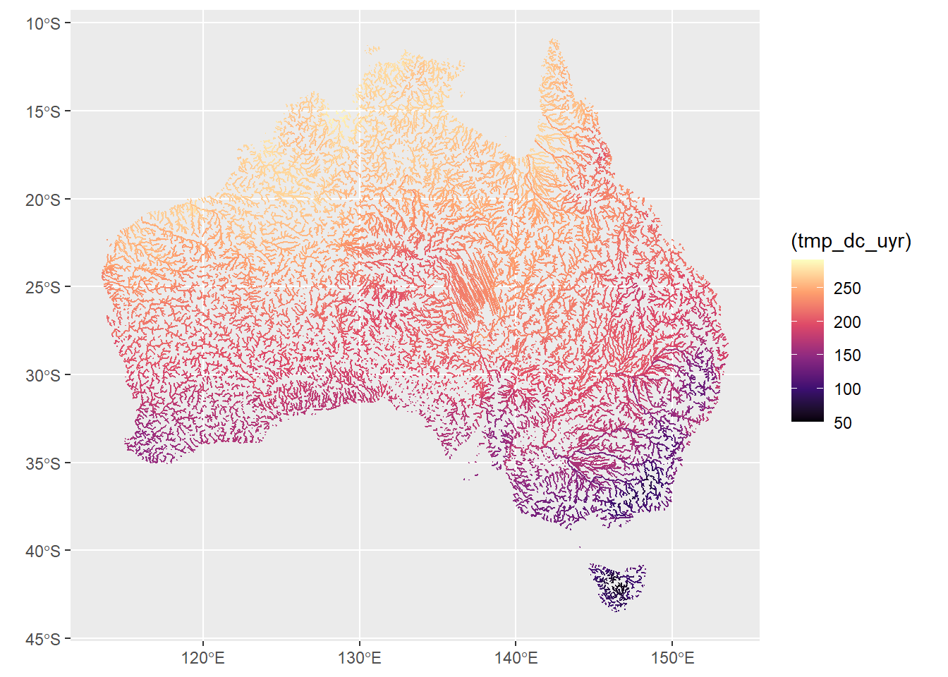

Discharge

ggplot() +
  geom_sf(data = aus_rivers |> filter(ORD_STRA >= 3), mapping = aes(color = dis_m3_pyr)) +
  scale_color_viridis_c(option = 'mako', trans = 'log10')

Warning in scale_color_viridis_c(option = "mako", trans = "log10"): log-10
transformation introduced infinite values.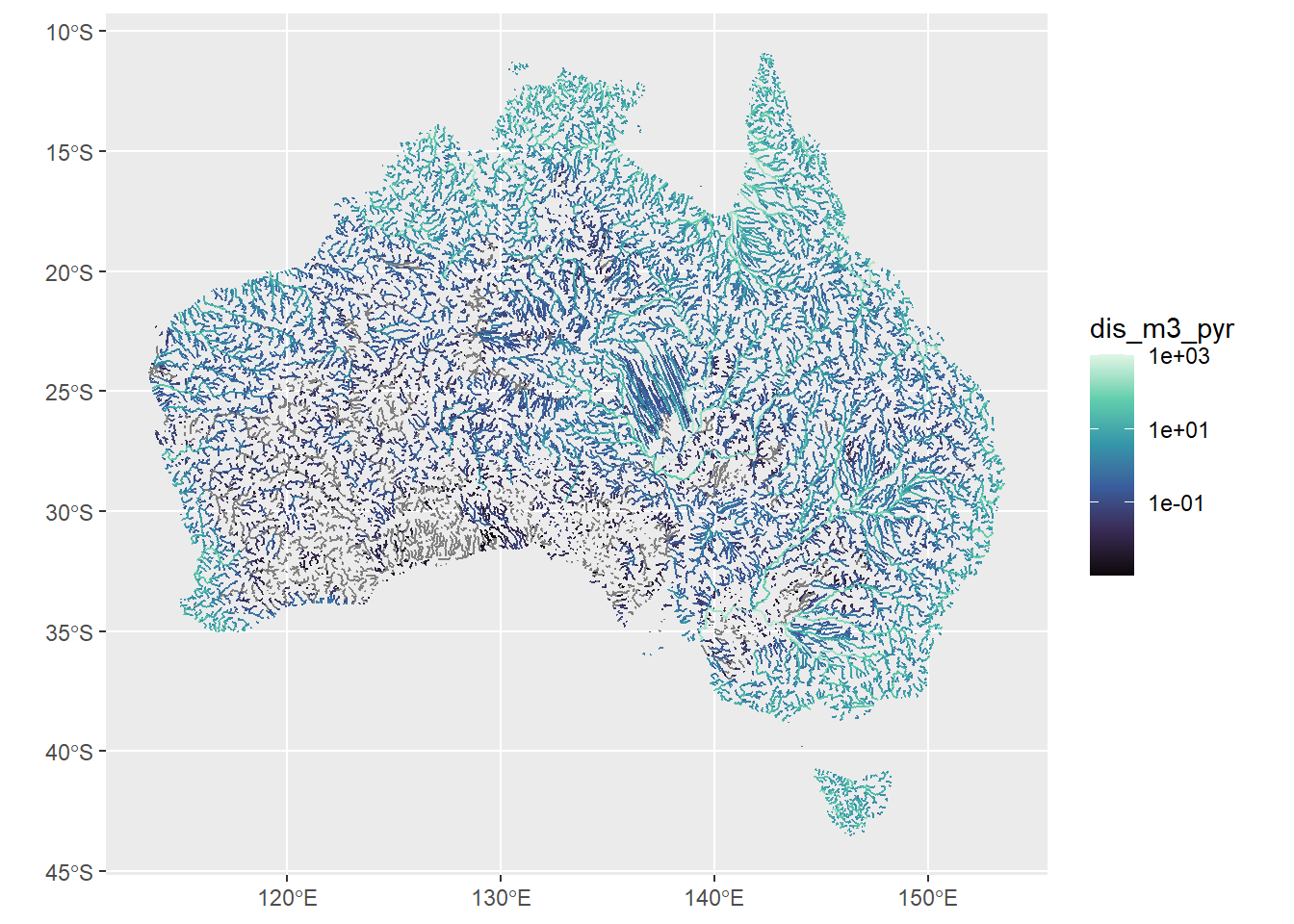

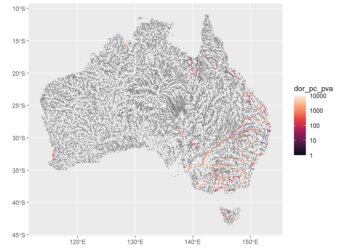
Regulation

ggplot() +
  geom_sf(data = aus_rivers |> filter(ORD_STRA >= 3), mapping = aes(color = dor_pc_pva)) +
  scale_color_viridis_c(option = 'rocket', trans = 'log10')

Warning in scale_color_viridis_c(option = "rocket", trans = "log10"): log-10
transformation introduced infinite values.