library(ggforce)
library(tidyverse)
devtools::load_all()
ℹ Loading galenRI need to create something like a Venn diagram, but scaled. None of the venn packages seem to do it. Can I get it to work with geom_circle and some math?
library(ggforce)
library(tidyverse)
devtools::load_all()ℹ Loading galenRFirst, let’s say we have two sets of different size, with some overlap
set1 <- 1:100
set2 <- 75:125
If we want to just represent each set as a circle with area proportional to the number of items and not worrying about overlap, we can
cirtib <- tibble(set_num = c(1,2), set_size = c(length(set1), length(set2))) |>
mutate(set_r = sqrt(set_size/pi))ggplot(cirtib) +
geom_circle(mapping = aes(x0 = 0, y0 = 0,
r = set_r,
color = factor(set_num))) +
coord_fixed()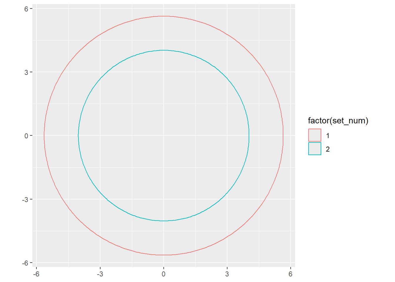
Now, though, I want an area of overlap of 25. So really, I need to find an offset for (let’s say) x0 for set2 that shifts that circle half in and half out.
Wolfram has a complicated formula (14) to get A (the area of the ‘lens’- the overlap) given the distance d between centers and the radii. Here, we have the area and radii, and want to solve for d. So can we do that?
A = r^2*acos((d^2 + r^2 - R^2) / (2*d*r)) +
  R^2*acos((d^2 - r^2 + R^2) / (2*d*r)) -
  0.5*sqrt((d+r-R) * (d-r+R) * (-d+r+r) * (d+r+R))
According to Sage
pi - acos(-1/2*(R^2 - d^2 - r^2)/(d*r)) == 1/2*(2*(pi - acos(-1/2*(R^2 + d^2 - r^2)/(d*r)))*R^2 + 2*pi*r^2 - 2*A - sqrt(R^3*d + R^2*d^2 - R*d^3 - d^4 + (2*R - d)*r^3 - 2*r^4 + (2*R^2 + 3*R*d + 3*d^2)*r^2 - (2*R^3 + 3*R^2*d - d^3)*r))/r^2That’s not particularly helpful; d is not isolated.
I should be able to just do this numerically with optim or optimize, I think.
# calc_a <- function(d, radius1, radius2) {
#   A <- radius1^2*acos((d^2 + radius1^2 - radius2^2) / (2*d*radius1)) +
#     radius2^2*acos((d^2 - radius1^2 + radius2^2) / (2*d*radius1)) -
#     0.5*sqrt((d+radius1-radius2) * (d-radius1+radius2) * (-d+radius1+radius1) * (d+radius1+radius2))
#
#   return(A)
# }
#
# opt_d <- function(d, area, radius1, radius2) {
#
#   dcheck <- calc_a(d, radius1, radius2)
#
#   return(dcheck - area)
# }
# get the optimal shift
#opt_d and calc_a are defined in venn_distances.R
# find_d <- function(area, radii, radius1, radius2) {
# if (!missing(radii) & (!missing(radius1) | !missing(radius2))) {
# rlang::abort('either use radii or radius1, radius2')
# }
#
# if (missing(radii)) {
# radii <- c(radius1, radius2)
# }
# bestd <- optimize(opt_d, lower = abs(diff(radii)), upper = sum(radii),
# area = area, radii = radii)
# }# need to get this into the mutate somehow
d <- find_d(area = length(intersect(set1, set2)), radii = cirtib$set_r)
cirtib$set_d = c(0, d)ggplot(cirtib) +
geom_circle(mapping = aes(x0 = set_d, y0 = 0,
r = set_r,
color = factor(set_num))) +
coord_fixed()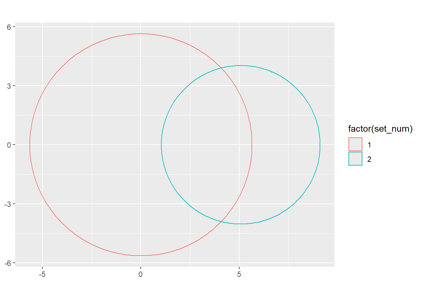
To get that to work with a mutate, we need to feed it both radii. we could do that long or wide, but given that we usually have long data:
Make a column identifying the set, another with the set intersection, and use that to make the d in a grouped mutate.
cirtib <- cirtib |>
  mutate(setpair = 1,
         overlap = length(intersect(set1, set2))) |>
  mutate(setd_tidy = find_d(unique(overlap), set_r), .by = setpair) |>
  # we don't want to shift BOTH circles. If we want them centered, we can shift +- half
mutate(centers = setd_tidy*c(-0.5, 0.5))ggplot(cirtib) +
geom_circle(mapping = aes(x0 = centers, y0 = 0,
r = set_r,
fill = factor(set_num)),
alpha = 0.4) +
coord_fixed()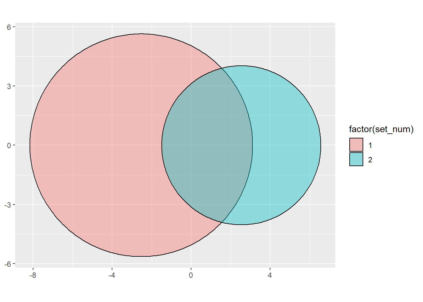
That really is fairly contrived to have the separate circles long. But when it comes time to plot, it’s WAY nicer.
Let’s say we have a dataset where we have already calculated the sizes and overlaps of a bunch of sets. Just make it long, since that’s how the data we want to use will be, and it makes the plotting easier.
manysets <- tibble(set_pair = rep(1:11, each = 2),
                   set_num = rep(1:2, 11),
                   area= runif(22)*100) |>
  mutate(overlapfrac = rep(seq(0, 1, 0.1), each = 2)) |>
  mutate(overlap = overlapfrac*min(area), .by = set_pair)
Now, to make the circles, we need to calculate radii and distance between centers. This is now equally as annoyign to be wide
manysets <- manysets |>
  mutate(radius = sqrt(area/pi)) |>
  mutate(d = find_d(unique(overlap), radii = radius), .by = set_pair)

# makes testing easier
manysets <- manysets |>
  # and a check
  mutate(area_calc = calc_a(unique(d), radii = radius), .by = set_pair) |>
  mutate(area_error = abs(overlap - area_calc)) |>
  mutate(centers = d*c(-0.5, 0.5))
Now to plot
ggplot(manysets) +
  geom_circle(mapping = aes(x0 = centers, y0 = (set_pair-1)*10,
                            r = radius,
                            fill = factor(set_num)),
              alpha = 0.4) +
  coord_fixed()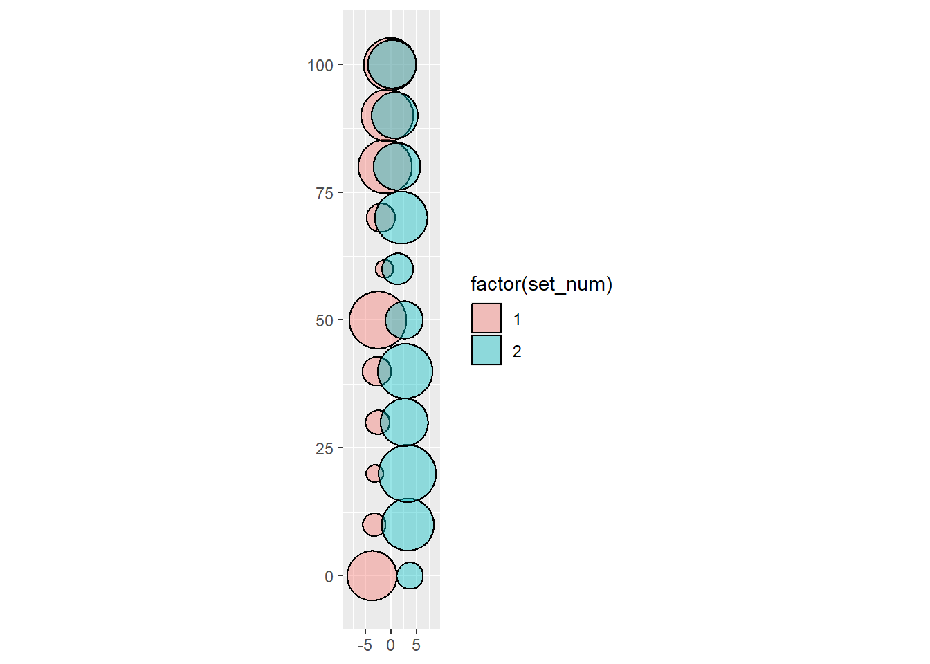
And the area_error is always very low
manysets# A tibble: 22 × 10
set_pair set_num area overlapfrac overlap radius d area_calc area_error
<int> <int> <dbl> <dbl> <dbl> <dbl> <dbl> <dbl> <dbl>
1 1 1 73.7 0 0 4.84 7.42 0.00000176 0.00000176
2 1 2 20.8 0 0 2.58 7.42 0.00000176 0.00000176
3 2 1 15.8 0.1 1.58 2.24 6.56 1.58 0.0000554
4 2 2 81.7 0.1 1.58 5.10 6.56 1.58 0.0000554
5 3 1 8.83 0.2 1.77 1.68 6.36 1.77 0.0000764
6 3 2 98.5 0.2 1.77 5.60 6.36 1.77 0.0000764
7 4 1 17.3 0.3 5.20 2.35 5.21 5.20 0.0000348
8 4 2 67.5 0.3 5.20 4.63 5.21 5.20 0.0000348
9 5 1 24.9 0.4 9.96 2.81 5.55 9.96 0.0000984
10 5 2 89.7 0.4 9.96 5.34 5.55 9.96 0.0000984
# ℹ 12 more rows
# ℹ 1 more variable: centers <dbl>The way this work is probably easier to see not with random sizes, but consistent
evensets <- tibble(set_pair = rep(1:11, each = 2),
                   set_num = rep(1:2, 11),
                   area = rep(c(100, 50), 11)) |>
  mutate(overlapfrac = rep(seq(0, 1, 0.1), each = 2)) |>
  mutate(overlap = overlapfrac*min(area), .by = set_pair)
Now get r, d, and centers
evensets <- evensets |>
  mutate(radius = sqrt(area/pi)) |>
  mutate(d = find_d(unique(overlap), radii = radius), .by = set_pair) |>
  mutate(centers = d*c(-0.5, 0.5))

# makes testing easier
evensets <- evensets |>
  # and a check
  mutate(area_calc = calc_a(unique(d), radii = radius), .by = set_pair) |>
  mutate(area_error = abs(overlap - area_calc))
Now to plot
ggplot(evensets) +
  geom_circle(mapping = aes(x0 = centers, y0 = (set_pair-1)*12,
                            r = radius,
                            fill = factor(set_num)),
              alpha = 0.4) +
  coord_fixed()
One thing I’m going to want to do when I use this is scale them (e.g. I’ll have massive numbers, but need to scale them down). I think the easiest way to do that is to just operate on scaled areas and overlaps.
So, recapitulating the above but with larger numers and then scaled
scaledsets <- tibble(set_pair = rep(1:11, each = 2),
                   set_num = rep(1:2, 11),
                   area = rep(c(10000, 5000), 11)) |>
  mutate(overlapfrac = rep(seq(0, 1, 0.1), each = 2)) |>
  mutate(overlap = overlapfrac*min(area), .by = set_pair) |>
  mutate(area_scaled = area/100, overlap_scaled = overlap/100)
Now get r, d, and centers
scaledsets <- scaledsets |>
  mutate(radius = sqrt(area/pi),
         radius_scaled = sqrt(area_scaled/pi)) |>
  mutate(d = find_d(unique(overlap), radii = radius),
         d_scaled = find_d(unique(overlap_scaled), radii = radius_scaled),
         .by = set_pair) |>
  mutate(centers = d*c(-0.5, 0.5),
         centers_scaled = d_scaled*c(-0.5, 0.5))
Now to plot First the raw
ggplot(scaledsets) +
  geom_circle(mapping = aes(x0 = centers, y0 = (set_pair-1)*12,
                            r = radius,
                            fill = factor(set_num)),
              alpha = 0.4) +
  coord_fixed()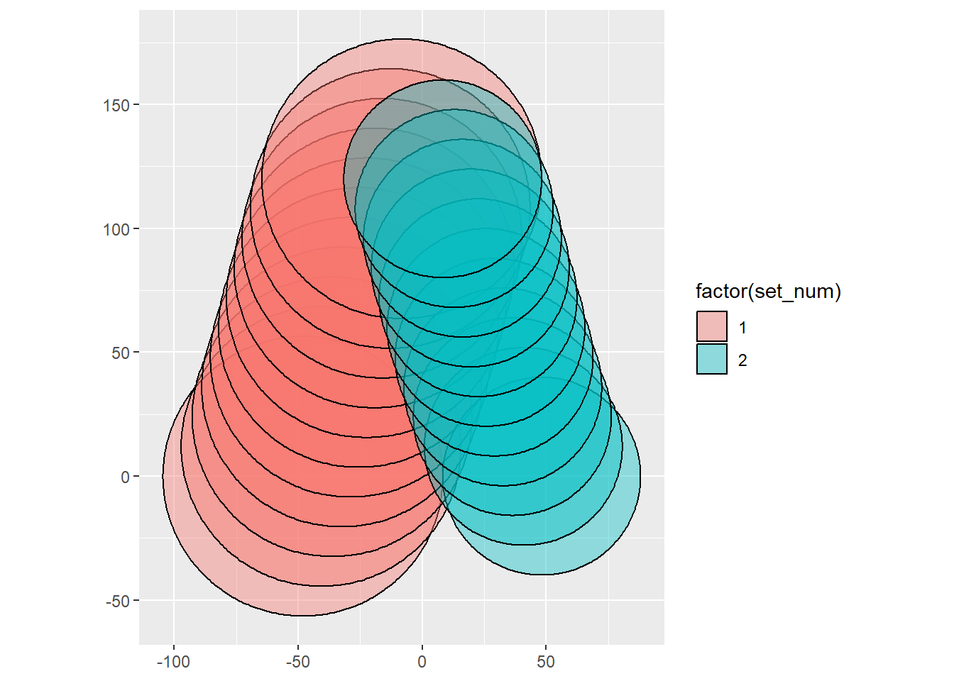
Then the scaled, looks like before.
ggplot(scaledsets) +
  geom_circle(mapping = aes(x0 = centers_scaled, y0 = (set_pair-1)*12,
                            r = radius_scaled,
                            fill = factor(set_num)),
              alpha = 0.4) +
  coord_fixed()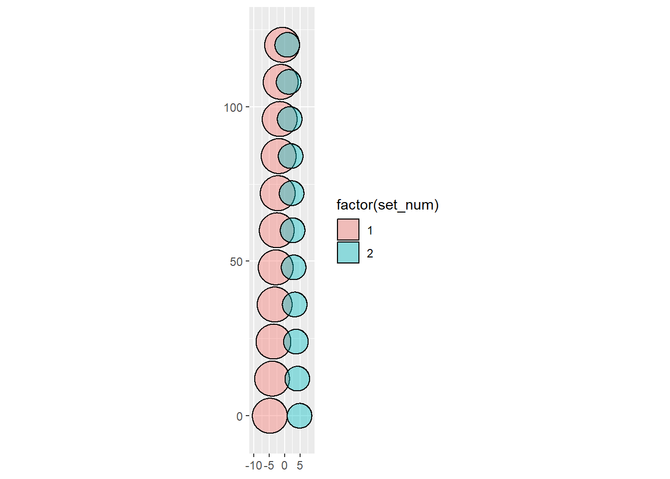
Now, if the goal is just to plot, can I (should I) write a little function that just returns radii and centers? It would require a very specific data format, so not sure it’s worth it. Obviously it could be generalised to long, wide, and as here, partially-long (areas in col, but overlap in another). I think I might see how useful it would be when I actually try to do this for my data and then decide
We could also use d to go in any direction, with any offset. E.g. from a base 0,0, we could shift only one circle right or left or up or down or given an angle and pythagoras off at an arbitrary angle.