At present, we largely assume the user will have a list of gauges
they want. The KiWIS interface does provide some opportunity to
programatically find gauge numbers according to criteria, using
getParameterList(), getGroupList(), and
getStationList() (most useful). This vignette, however,
assumes we have selected a set of gauges and want to identify variables
and pull their timeseries. For experimental wrappers that abstract some
of this, see their
vignette.
Unlike Hydstra, which provides tailored arguments for different sorts
of API control, KiWIS primarily uses text search within columns. This
can be more flexible, but means we need to know column names and pay
close attention to the regex used to filter those columns to avoid
contaminating outputs. This generality means that no column is favoured
over others in filtering, and hydrogauge provides access to the full
search capability with the extra_list argument. However, we
also make a concession for consistency by making station_no
its own argument, corresponding to the site_list argument
in Hydstra.
Querying available data
To get timeseries, the user needs to ask for specific variables and
timespans. Sometimes these are known a priori, e.g. if a gauge
was chosen because it is known to have flow for a desired period.
However, finding available variables and their periods of record can
also be done through the functions here, primarily
getTimeseriesList(). This is one of the main purposes of
this package; we want to be able to query available data.
Finding available variables and timespans
Due to the search functionality of the KiWIS interface, we can use
gauge numbers as we do with hydstra, but we can also search more
generally. Note also that this returns a very large list, primarily due
to the values in ts_id and ts_name columns,
which arise because the various types of data and aggregations are given
unique values there, rather than being calculated, as they are for
hydstra.
station_tslist <- getTimeseriesList(portal = 'bom', station_no = c('410730', 'A4260505'))

station_tslist
#> # A tibble: 200 × 14
#>    station_name    station_no station_id ts_id ts_name ts_unitname ts_unitsymbol
#>    <chr>           <chr>      <chr>      <chr> <chr>   <chr>       <chr>
#>  1 River Murray a… A4260505   1617110    2086… Receiv… cubic mete… cumec
#>  2 River Murray a… A4260505   1617110    2086… Harmon… cubic mete… cumec
#>  3 River Murray a… A4260505   1617110    2086… DMQaQc… cubic mete… cumec
#>  4 River Murray a… A4260505   1617110    2086… DMQaQc… meter       m
#>  5 River Murray a… A4260505   1617110    2086… DMQaQc… meter       m
#>  6 River Murray a… A4260505   1617110    2086… Harmon… cubic mete… cumec
#>  7 River Murray a… A4260505   1617110    2086… Harmon… meter       m
#>  8 River Murray a… A4260505   1617110    2086… Receiv… meter       m
#>  9 River Murray a… A4260505   1617110    2086… Combin… meter       m
#> 10 River Murray a… A4260505   1617110    2086… DMQaQc… meter       m
#> # ℹ 190 more rows
#> # ℹ 7 more variables: ts_path <chr>, parametertype_id <chr>,
#> #   parametertype_name <chr>, stationparameter_name <chr>, from <dttm>,
#> #   to <dttm>, database_timezone <chr>
We can visualise the time period for each parameter at each gauge (here limited only to the QA’ed daily means).
station_tslist |>
  dplyr::filter(grepl('DMQaQc.Merged.DailyMean.24HR', ts_name)) |>
  tidyr::pivot_longer(cols = c(from, to), names_to = 'startend', values_to = 'date') |>
ggplot(aes(y = date, x = station_no, color = parametertype_name)) +
  geom_point(position = position_dodge(width = 0.5)) +
  geom_line(position = position_dodge(width = 0.5)) +
  coord_flip()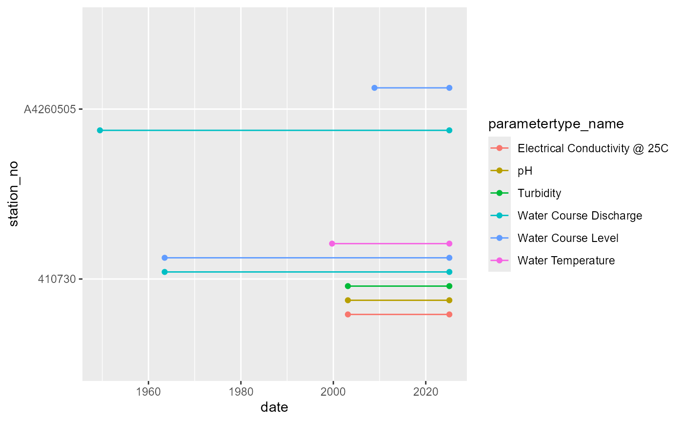
Availability of each variable at each gauge, with the period of record indicated by lines.
We can take advantage of the search capability to ignore gauge
numbers entirely, returning all sites meeting some regex pattern, here
those with 'River Murray' in the station_name.
We do this with the extra_list argument, which takes column
names as names and the seach pattern as the item. This approach works
for any column, and so we also only look at the “DMQaQc” data at a Daily
Mean aggregation. The returnfields argument lets us choose
which columns to return. We include ‘coverage’ here to the returnfields
to get the period of record.
RM_ts <- getTimeseriesList(portal = 'bom',
                           extra_list = list(station_name = 'River Murray*',
                                             ts_name = 'DMQaQc.Merged.DailyMean.24HR'),
                           returnfields = c('station_no', 'station_name',
                                            'ts_name', 'ts_id',
                                            'ts_unitname', 'parametertype_name',
                                            'coverage'))

RM_ts
#> # A tibble: 199 × 9
#>    station_no station_name          ts_name ts_id ts_unitname parametertype_name
#>    <chr>      <chr>                 <chr>   <chr> <chr>       <chr>
#>  1 A4260573   River Murray at Wool… DMQaQc… 2107… degree Cel… Water Temperature
#>  2 A4260624   River Murray at Love… DMQaQc… 2118… meter       Water Course Level
#>  3 A4260632   River Murray at Temp… DMQaQc… 2121… meter       Water Course Level
#>  4 A4260643   River Murray at Habe… DMQaQc… 2124… microsieme… Electrical Conduc…
#>  5 A4260507   River Murray at Lock… DMQaQc… 2087… meter       Water Course Level
#>  6 A4260509   River Murray at Lock… DMQaQc… 2087… microsieme… Electrical Conduc…
#>  7 A4260521   River Murray at Mann… DMQaQc… 2091… microsieme… Electrical Conduc…
#>  8 A4260522   River Murray at Murr… DMQaQc… 2092… meter       Water Course Level
#>  9 A4260522   River Murray at Murr… DMQaQc… 2092… degree Cel… Water Temperature
#> 10 A4260532   River Murray at Well… DMQaQc… 2097… meter       Water Course Level
#> # ℹ 189 more rows
#> # ℹ 3 more variables: from <dttm>, to <dttm>, database_timezone <chr>
We can visualise the availability of each variable at each gauge (@ref(fig:vars-duration)).
RM_ts |>
  dplyr::mutate(duration = to-from) |>
ggplot(aes(x = parametertype_name, y = station_no, fill = duration)) +
  geom_tile() +
  scale_fill_viridis_c(option = 'plasma') +
  theme(axis.text.x = element_text(angle = 45, hjust = 1))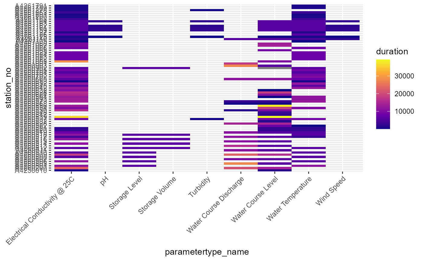
Availability of each variable at each gauge, with color indicating the duration of record in days.
The available returnfields are poorly documented. The default are
those returned above for station_tslist,
names(station_tslist)[!names(station_tslist) %in% c('from', 'to', 'database_timezone')]
#>  [1] "station_name"          "station_no"            "station_id"
#>  [4] "ts_id"                 "ts_name"               "ts_unitname"
#>  [7] "ts_unitsymbol"         "ts_path"               "parametertype_id"
#> [10] "parametertype_name"    "stationparameter_name"
But there are others that can be requested. In particular, ‘coverage’ is needed to get the period of record.
  # According to kisters, these exist
  all_return <- c('station_name', 'station_latitude', 'station_longitude', 'station_carteasting', 'station_cartnorthing', 'station_local_x', 'station_local_y', 'station_georefsystem', 'station_longname', 'ts_id', 'ts_name', 'ts_shortname', 'ts_path', 'ts_type_id', 'ts_type_name', 'parametertype_id', 'parametertype_name', 'stationparameter_name', 'stationparameter_no', 'stationparameter_longname', 'ts_unitname', 'ts_unitsymbol', 'ts_unitname_abs', 'ts_unitsymbol_abs', 'site_no', 'site_id', 'site_name', 'catchment_no', 'catchment_id', 'catchment_name', 'coverage', 'ts_density', 'ts_exchange', 'ts_spacing', 'ts_clientvalue##', 'datacart', 'ca_site', 'ca_sta', 'ca_par', 'ca_ts')
  # I get http 500 errors unless cut to
  sub_return <- all_return[c(1:34, 37:40)]
  sub_return
#>  [1] "station_name"              "station_latitude"
#>  [3] "station_longitude"         "station_carteasting"
#>  [5] "station_cartnorthing"      "station_local_x"
#>  [7] "station_local_y"           "station_georefsystem"
#>  [9] "station_longname"          "ts_id"
#> [11] "ts_name"                   "ts_shortname"
#> [13] "ts_path"                   "ts_type_id"
#> [15] "ts_type_name"              "parametertype_id"
#> [17] "parametertype_name"        "stationparameter_name"
#> [19] "stationparameter_no"       "stationparameter_longname"
#> [21] "ts_unitname"               "ts_unitsymbol"
#> [23] "ts_unitname_abs"           "ts_unitsymbol_abs"
#> [25] "site_no"                   "site_id"
#> [27] "site_name"                 "catchment_no"
#> [29] "catchment_id"              "catchment_name"
#> [31] "coverage"                  "ts_density"
#> [33] "ts_exchange"               "ts_spacing"
#> [35] "ca_site"                   "ca_sta"
#> [37] "ca_par"                    "ca_ts"
Obtaining timeseries
To pull timeseries, we need to know either the ts_id or
ts_path arguments that we want. This filters on those
columns to ensure we get the timeseries we want. Note in both
station_tslist and RM_ts that each row
(defined by station, variable, aggregation, QA’d, etc) gets its own
ts_id value. We need to choose the ones we want.
The find_ts_id() function helps us find desired ts_id
values. It is a wrapper over getTimeseriesList() with regex
to select what we want. As such, it’s not in the raw API workflow, but
is very handy. See the
wrapper vignette
In choosing these ts_ids, we’re making many of the same
decisions we would make when asking the hydstra function
get_ts_traces() for site_list,
datasource, var_list, interval,
data_type, and multiplier. This has pluses and
minuses. It’s much harder here to ask for what we want (but see
find_ts_ids()), but because each aggregation is
pre-supplied and indexed uniquely it’s much easier to get different
aggregations from different variables in one call.
Let’s demonstrate with some ts_id values from
station_tslist to pull daily mean QaQc’ed values for level,
discharge, and water temp. Note that we have to ask for discharge and
level with separate ts_ids for each gauge. This is another argument for
using find_ts_id().
ts_example <- c(
  '208669010', '208648010', # level and discharge Lock 9
  '1573010', '1598010', # level and discharge Cotter R.
  '380167010'
  )
We’ll just pull one year
ts_example <- getTimeseriesValues(portal = 'bom',
                                  ts_id = ts_example,
                                  start_time = 20100101,
                                  end_time = 20101231)
That provides a tall dataframe containing additional information
about the gauge (@tbl-ts). The returned
columns can again be adjusted with returnfields and
meta_returnfields.
# rows.print doesn't really work with devtools::build_readme(), so use head
head(ts_example, 30)
#> # A tibble: 30 × 14
#>    ts_id     station_name  station_latitude station_longitude parametertype_name
#>    <chr>     <chr>         <chr>            <chr>             <chr>
#>  1 208648010 River Murray… ""               ""                Water Course Disc…
#>  2 208648010 River Murray… ""               ""                Water Course Disc…
#>  3 208648010 River Murray… ""               ""                Water Course Disc…
#>  4 208648010 River Murray… ""               ""                Water Course Disc…
#>  5 208648010 River Murray… ""               ""                Water Course Disc…
#>  6 208648010 River Murray… ""               ""                Water Course Disc…
#>  7 208648010 River Murray… ""               ""                Water Course Disc…
#>  8 208648010 River Murray… ""               ""                Water Course Disc…
#>  9 208648010 River Murray… ""               ""                Water Course Disc…
#> 10 208648010 River Murray… ""               ""                Water Course Disc…
#> # ℹ 20 more rows
#> # ℹ 9 more variables: ts_name <chr>, ts_unitname <chr>, ts_unitsymbol <chr>,
#> #   station_no <chr>, station_id <chr>, value <dbl>, quality_code <int>,
#> #   time <dttm>, database_timezone <chr>
ts_example |>
  ggplot(aes(x = time, y = value, color = parametertype_name)) +
  geom_line() +
  facet_grid(parametertype_name ~ station_name, scales = 'free', labeller = label_wrap_gen(10))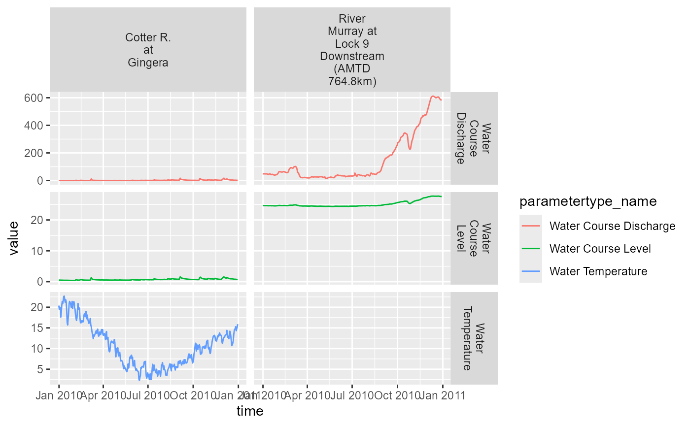
Timeseries of requested data, where available.
A common use will be asking for the period of record, so we show that
here for these two gauges. We use the period = 'complete'
argument to take advantage of internal API functionality (which also
allows period units like ‘P2W’).
ts_all <- getTimeseriesValues(portal = 'bom',
                                  ts_id = c('208648010', '1573010'),
                                  period = 'complete')
ts_all |>
  # dplyr::filter(value >= 0) |>
  ggplot(aes(x = time, y = value, color = station_name)) +
  geom_line() +
  facet_grid(station_name ~ ., scales = 'free', labeller = label_wrap_gen(10)) +
  theme(legend.position = 'none')
#> Warning: Removed 4 rows containing missing values or values outside the scale range
#> (`geom_line()`).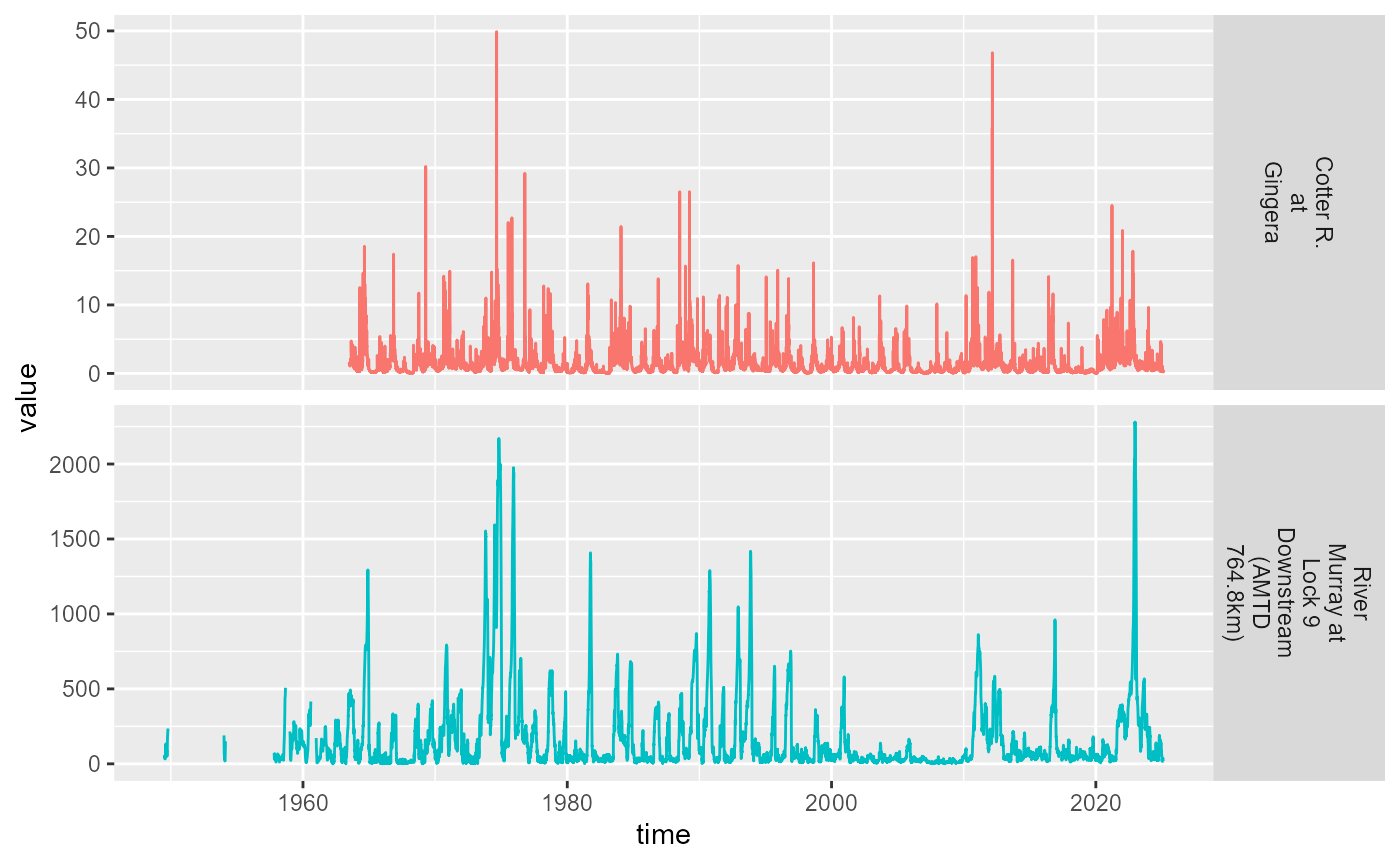
Timeseries of period of record for discharge.
An automated approach that can simplify some common workflows
(especially pulling period of record for many gauges and programatically
selecting variables across gauges) is available in
fetch_kiwis_timeseries(). See the
article.