At present, we largely assume the user will have a list of gauges
they want, as the current ability to programatically obtain gauge
numbers according to criteria is limited (but see
get_sites_by_datasource(), which allows asking for all
sites that have a given datasource). This vignette walks through the
process with the core functions, for experimental wrappers that abstract
some of this, see their
vignette.
To get timeseries, the user needs to ask for specific variables and timespans. Sometimes these are known a priori, e.g. if a gauge was chosen because it is known to have flow for a desired period. However, finding available variables and their periods of record can also be done through the functions here. This is one of the main purposes of this package; we want to be able to query available data.
This vignette will proceed with a set of sites chosen to span a range of characteristics useful for this demonstration.
The Upper Steavenson (405328) only has flow
Barwon (233217) has many variables, but their start dates differ
Taggerty (405331) is no longer in operation- ran 2010-2013
Marysville golf course (405837) is only rainfall
The functions all require gauges to be their numeric codes as
characters. The API needs a comma-separated string
("number1, number2" ) , but the functions here will accept
a vector c("number1", "number2") and decompose it
internally. This is typically easier and reflects more common R
workflows such as having a column of site numbers in a dataframe.
barwon <- '233217'
steavenson <- '405328'
taggerty <- '405331'
golf <- '405837'
Querying available data
Before asking for timeseries data, we want to ask what data is available. we use
Finding datasources
To see what datasources are available for a site, use
get_datasources_by_site(). I typically use “A”, but it’s
worth looking to see what datasources are available for a target
site(s), and then doing the next step (finding variables) for each, to
see whether the available variables (or timeperiods) differ. Note-
there are often other datasources that work but are not returned
here.
ds <- get_datasources_by_site(portal = 'Vic',
                              site_list = c(barwon, steavenson,
                                            taggerty, golf))
ds
#> # A tibble: 10 × 2
#>    site   datasource
#>    <chr>  <chr>
#>  1 233217 A
#>  2 233217 TELEM
#>  3 233217 TELEMCOPY
#>  4 405328 A
#>  5 405328 TELEM
#>  6 405328 TELEMCOPY
#>  7 405331 A
#>  8 405837 A
#>  9 405837 TELEM
#> 10 405837 TELEMCOPY
Plot that to see data availability (@ref(fig:datasource)).
plot_datasources_by_site(ds)
#> Joining with `by = join_by(site, datasource)`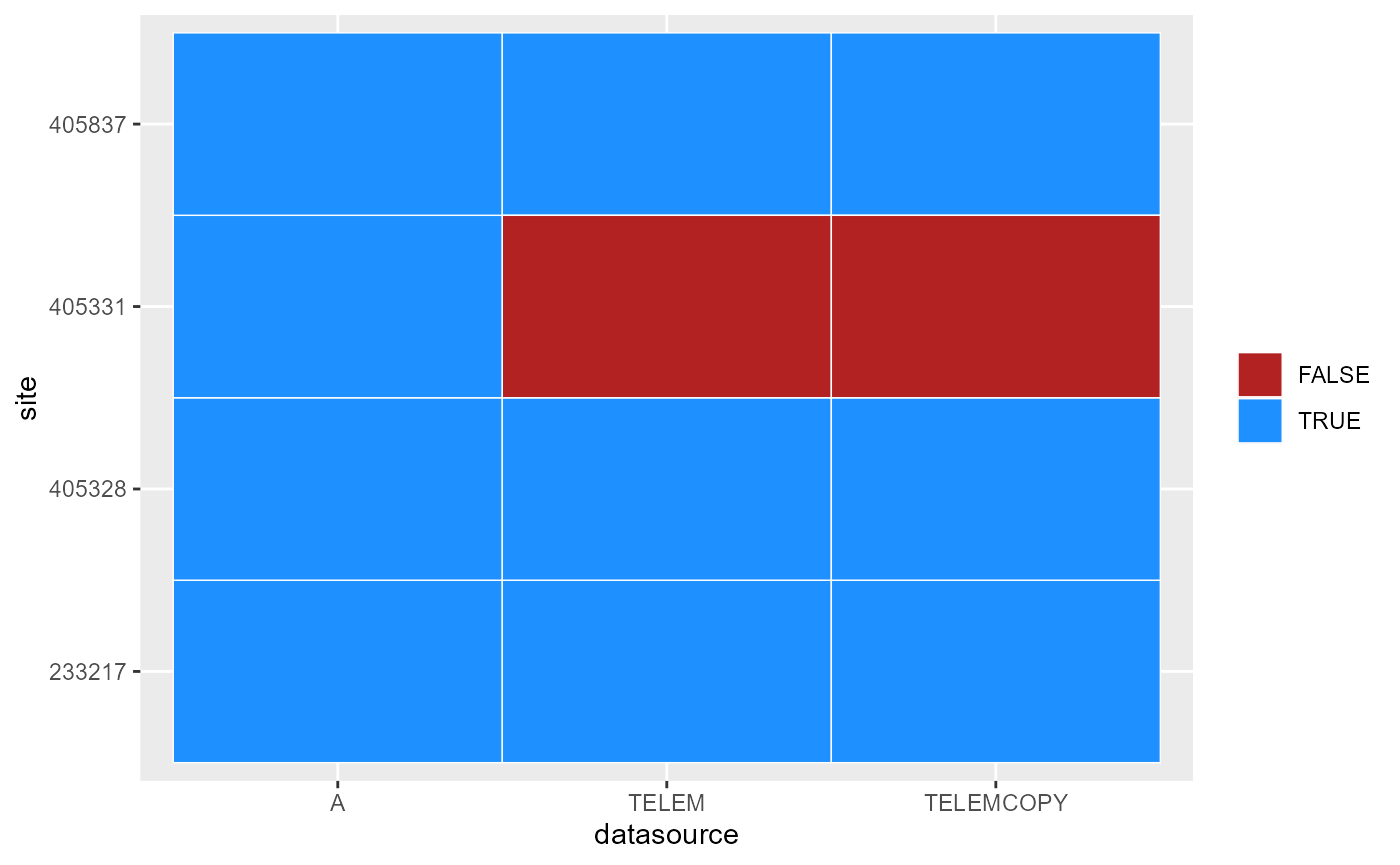
Datasources available for each gauge. These are what are returned by the API, but may not be complete. Specifying other datasources on a pull may work.
Finding available variables and timespans
We then need to know what variables are available to extract
timeseries of. We use get_variable_list() to get this
information, including both their names and numbers, as well as other
details such as the time period of record and units.
var_info <- get_variable_list(portal = 'Vic',
                              site_list = c(barwon, taggerty,
                                            steavenson, golf),
                              datasource = "A")
That returns a tibble with information about each gauge and variable (@tbl-vars). A few things to note- it gives the names of the gauges, the names and values of the variables, and a start and end date for each. For example, the Barwon’s start date for stage (100) is 1961, while the others (pH, ppm, etc) didn’t start until 2010.
Note that this does not return derived discharge variables (140 and 141). If variable 100 (stage height) exists, the other two usually do, though sometimes not if there is no ratings curve.
var_info
#> # A tibble: 12 × 11
#>    site   short_name       long_name variable units var_name period_start
#>    <chr>  <chr>            <chr>     <chr>    <chr> <chr>    <dttm>
#>  1 233217 BARWON @ GEELONG BARWON R… 100.00   metr… Stream … 1961-03-06 07:15:00
#>  2 233217 BARWON @ GEELONG BARWON R… 210.00   pH    Acidity… 2010-07-06 02:31:00
#>  3 233217 BARWON @ GEELONG BARWON R… 215.00   ppm   Dissolv… 2010-07-06 02:31:00
#>  4 233217 BARWON @ GEELONG BARWON R… 450.00   Degr… Water T… 2010-07-06 02:31:00
#>  5 233217 BARWON @ GEELONG BARWON R… 810.00   NTU   Turbidi… 2010-07-06 02:31:00
#>  6 233217 BARWON @ GEELONG BARWON R… 820.00   µS/c… Conduct… 2010-07-06 02:31:00
#>  7 405331 TAGGERTY R LADY… TAGGERTY… 100.00   metr… Stream … 2010-07-29 02:20:00
#>  8 405331 TAGGERTY R LADY… TAGGERTY… 450.00   Degr… Water T… 2010-07-29 02:20:00
#>  9 405331 TAGGERTY R LADY… TAGGERTY… 810.00   NTU   Turbidi… 2010-07-29 02:20:00
#> 10 405331 TAGGERTY R LADY… TAGGERTY… 820.00   µS/c… Conduct… 2010-07-29 02:20:00
#> 11 405328 STEAVENSON R @ … STEAVENS… 100.00   metr… Stream … 2009-11-19 07:08:00
#> 12 405837 R.G. MARYSVILLE  RAINGAUG… 10.00    mm    Rainfal… 2001-06-21 04:27:00
#> # ℹ 4 more variables: period_end <dttm>, subdesc <chr>, datasource <chr>,
#> #   database_timezone <chr>
Depending on the goals, it can be helpful to visualise this as the availability of each variable (@ref(fig:vars-duration)) or the period of record of each variable (@ref(fig:vars-period)).
var_info |>
  dplyr::mutate(duration = period_end-period_start) |>
ggplot(aes(x = var_name, y = site, fill = duration)) +
  geom_tile() +
  scale_fill_viridis_c(option = 'plasma') +
  theme(axis.text.x = element_text(angle = 45, hjust = 1))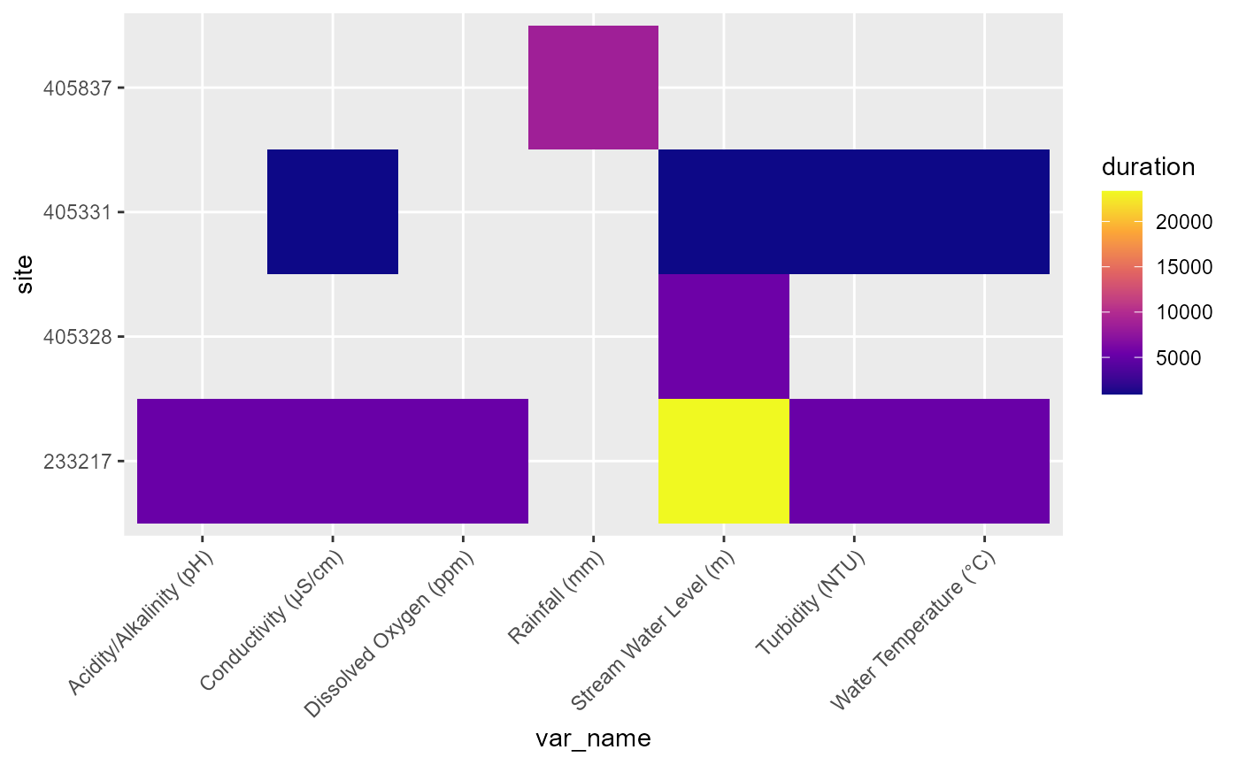
Availability of each variable at each gauge, with color indicating the duration of record in days.
var_info |>
  tidyr::pivot_longer(cols = starts_with('period'), names_to = 'startend', values_to = 'date') |>
ggplot(aes(y = date, x = site, color = var_name)) +
  geom_point(position = position_dodge(width = 0.5)) + geom_line(position = position_dodge(width = 0.5)) +
  coord_flip()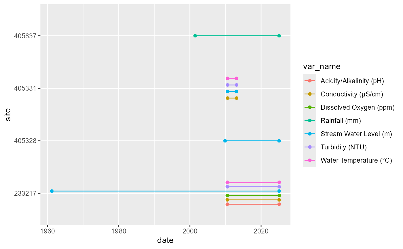
Availability of each variable at each gauge, with the period of record indicated by lines.
Obtaining timeseries
This is typically the main goal, with the other steps getting us to
the point of knowing what to ask for. Specifically,
get_variable_list() gives us a reference to know what the
variables are to ask for and the relevant timeperiods.
Basic operation
In general, we use get_ts_traces() for a set of sites,
variables, timeperiods, and statistics. The experimental wrapper
functions fetch_hydstra_timeseries() and
fetch_timeseries() call get_ts_traces()
internally. In any case, there are some pitfalls to avoid.
If we just want a set of variables that all need the same statistic applied (e.g. daily mean flows), we can pass that in as a vector. For example, to get daily mean stage height (100), discharge (here in ML/day, 141), and temperature (450), we can do that in one call, even for multiple gauges. Asking here for one year to keep the call quick.
ts_days <- get_ts_traces(portal = 'Vic',
                         site_list = c(barwon, steavenson, taggerty, golf),
                         datasource = "A",
                         var_list = c("100", "141", "450"),
                         start_time = 20200101,
                         end_time = 20201231,
                         interval = "day",
                         data_type = "mean",
                         multiplier = 1,
                         returnformat = 'df')
That returns a tall dataframe with both the requested values and some site metadata including the site name, location, etc (@tbl-ts), which the user can then split up or plot how they want (e.g. @ref(fig:ts)). There are other options that return lists of dataframes if the user does not want all sites and variables combined-
returnformat = "varlist"a list with one tibble per variablereturnformat = "sitelist"a list with one tibble per sitereturnformat = "sxvlist"a list with one tibble per site x variable combo (including empty lists for missing combos)
# rows.print doesn't really work with devtools::build_readme(), so use head
head(ts_days, 30)
#> # A tibble: 30 × 20
#>    error_num compressed site_short_name  longitude site_name   latitude org_name
#>        <int> <chr>      <chr>                <dbl> <chr>          <dbl> <chr>
#>  1         0 0          BARWON @ GEELONG      144. BARWON RIV…    -38.2 Dept. S…
#>  2         0 0          BARWON @ GEELONG      144. BARWON RIV…    -38.2 Dept. S…
#>  3         0 0          BARWON @ GEELONG      144. BARWON RIV…    -38.2 Dept. S…
#>  4         0 0          BARWON @ GEELONG      144. BARWON RIV…    -38.2 Dept. S…
#>  5         0 0          BARWON @ GEELONG      144. BARWON RIV…    -38.2 Dept. S…
#>  6         0 0          BARWON @ GEELONG      144. BARWON RIV…    -38.2 Dept. S…
#>  7         0 0          BARWON @ GEELONG      144. BARWON RIV…    -38.2 Dept. S…
#>  8         0 0          BARWON @ GEELONG      144. BARWON RIV…    -38.2 Dept. S…
#>  9         0 0          BARWON @ GEELONG      144. BARWON RIV…    -38.2 Dept. S…
#> 10         0 0          BARWON @ GEELONG      144. BARWON RIV…    -38.2 Dept. S…
#> # ℹ 20 more rows
#> # ℹ 13 more variables: value <dbl>, time <dttm>, quality_codes_id <int>,
#> #   site <chr>, variable_short_name <chr>, precision <chr>, subdesc <chr>,
#> #   variable <chr>, units <chr>, variable_name <chr>, database_timezone <chr>,
#> #   quality_codes <chr>, data_type <chr>
ts_days |>
  ggplot(aes(x = time, y = value, color = variable_short_name)) +
  geom_line() +
  facet_grid(variable_short_name ~ site_short_name, scales = 'free')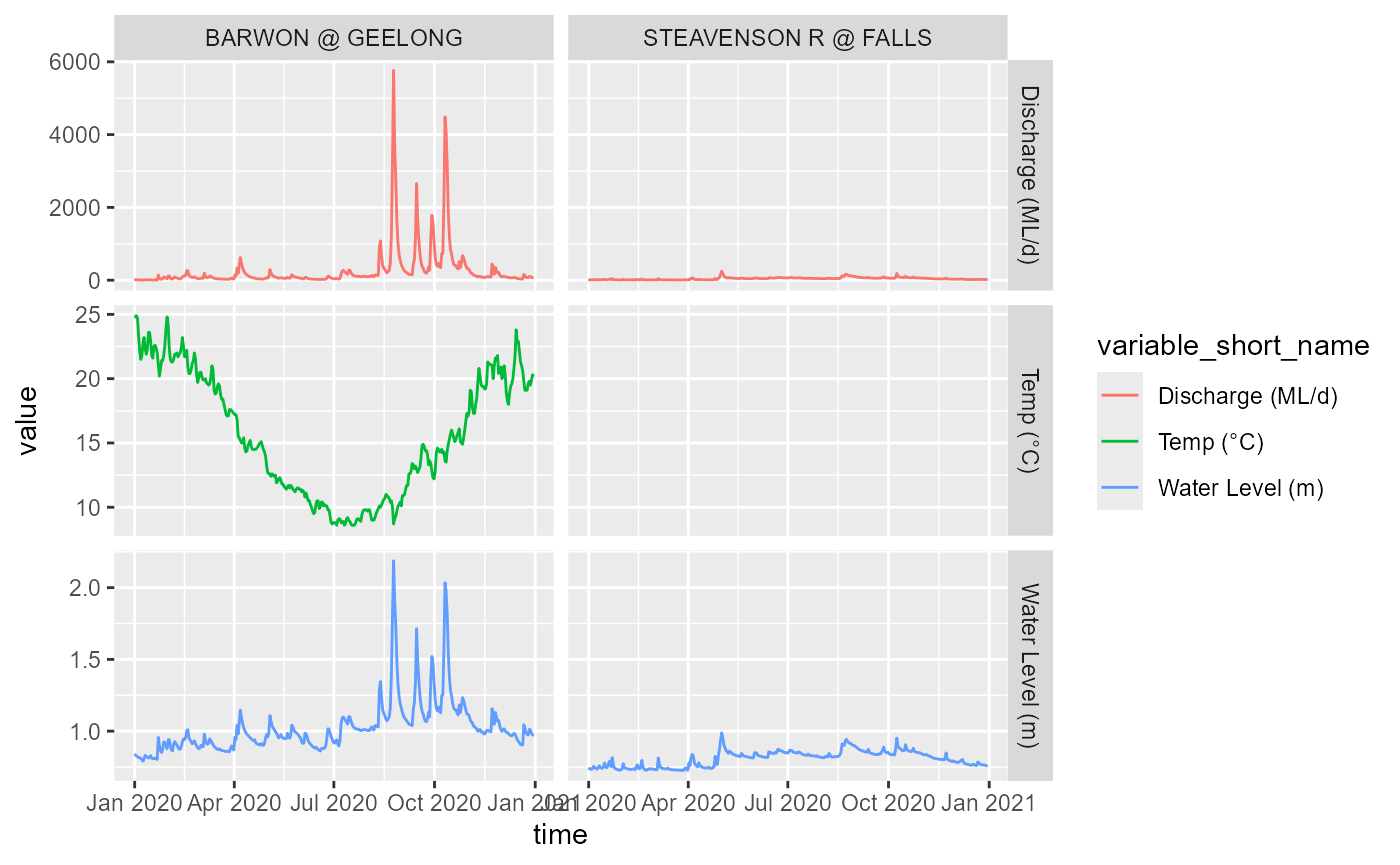
Timeseries of requested data, where available.
Note that if a variable isn’t available for a gauge it just isn’t returned, and same with timeperiods. We requested data from all four sites, but only the Barwon returns all variables. The golf course gauge does not return anything because it does not collect these variables, the Steavenson returns level and discharge but not temp, and the Taggerty doesn’t appear at all despite having these variables because we’ve asked for data after it was decommissioned.
Multiple variables, multiple statistics
Now, if we want another set of variables that should have a different
statistic (e.g. rainfall makes sense as the daily sum, not the mean), we
need a separate call to get_ts_traces() with a different
data_type argument.
Note that again this will ignore gauges without the info (@ref(tab:ts-rain-tab), @ref(fig:ts-rain-fig)).
ts_rain <- get_ts_traces(portal = 'Vic',
                         site_list = c(barwon, golf),
                         datasource = "A",
                         var_list = c("10"),
                         start_time = 20200101,
                         end_time = 20201231,
                         interval = "day",
                         data_type = "tot",
                         multiplier = 1,
                         returnformat = 'df')
head(ts_rain, 30)
#> # A tibble: 30 × 20
#>    error_num compressed site_short_name longitude site_name    latitude org_name
#>        <int> <chr>      <chr>               <dbl> <chr>           <dbl> <chr>
#>  1         0 0          R.G. MARYSVILLE      146. RAINGAUGE @…    -37.5 Dept. S…
#>  2         0 0          R.G. MARYSVILLE      146. RAINGAUGE @…    -37.5 Dept. S…
#>  3         0 0          R.G. MARYSVILLE      146. RAINGAUGE @…    -37.5 Dept. S…
#>  4         0 0          R.G. MARYSVILLE      146. RAINGAUGE @…    -37.5 Dept. S…
#>  5         0 0          R.G. MARYSVILLE      146. RAINGAUGE @…    -37.5 Dept. S…
#>  6         0 0          R.G. MARYSVILLE      146. RAINGAUGE @…    -37.5 Dept. S…
#>  7         0 0          R.G. MARYSVILLE      146. RAINGAUGE @…    -37.5 Dept. S…
#>  8         0 0          R.G. MARYSVILLE      146. RAINGAUGE @…    -37.5 Dept. S…
#>  9         0 0          R.G. MARYSVILLE      146. RAINGAUGE @…    -37.5 Dept. S…
#> 10         0 0          R.G. MARYSVILLE      146. RAINGAUGE @…    -37.5 Dept. S…
#> # ℹ 20 more rows
#> # ℹ 13 more variables: value <dbl>, time <dttm>, quality_codes_id <int>,
#> #   site <chr>, variable_short_name <chr>, precision <chr>, subdesc <chr>,
#> #   variable <chr>, units <chr>, variable_name <chr>, database_timezone <chr>,
#> #   quality_codes <chr>, data_type <chr>
ts_rain |>
  ggplot(aes(x = time, y = value, color = variable_short_name)) +
  geom_line() +
  facet_grid(variable_short_name ~ site_short_name, scales = 'free')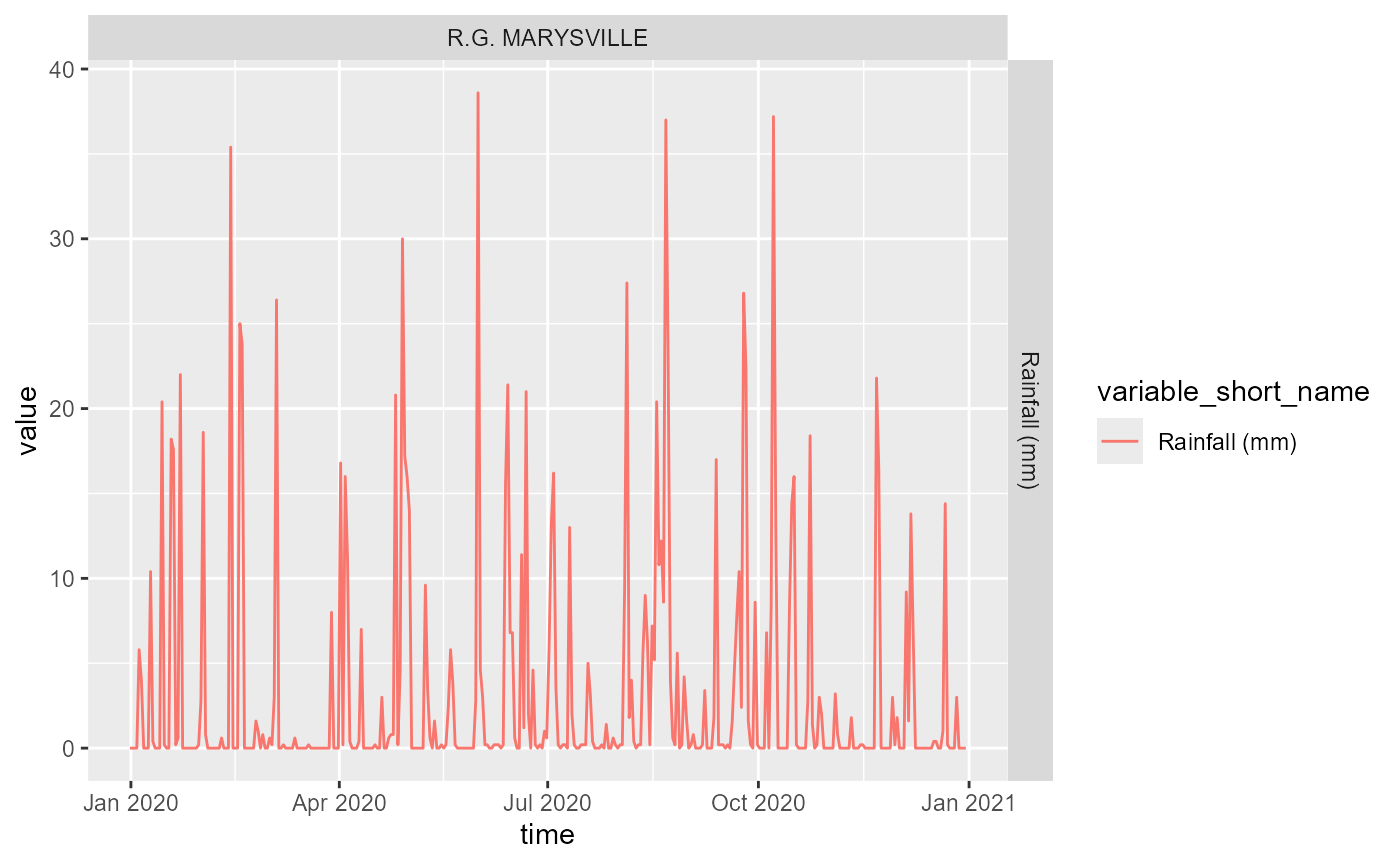
Timeseries of rainfall data, where available.
If the user wants to combine across different statistics, use
dplyr::bind_rows() to combine post-hoc.
An automated approach that can simplify some common workflows
(especially pulling period of record for many gauges) is available in
fetch_hydstra_timeseries(), but care must be taken to avoid
inappropriate statistics. See the
article.