xrange =c(0, 10)# we'll want this for predicting the fitsxdata <-tibble(x =seq(from =min(xrange), to =max(xrange), by =diff(xrange)/100))
This is essentially preamble to understanding the beta-binomial issues we’re having. But we should be able to do a better job sharpening our intuition of what we expect if we start off fully gaussian.
This builds on the outline I developed and the work Sarah did (students/Sarah_Taig/Random Effects Simulations) (though I think the emphasis will be different; we’ll see), as well as some beta-binom errorbar checks in caddis/Testing/Error_bars.qmd.
I think I’ll likely just do gaussian here. Then bb in a parallel doc. And likely will do a model comparison thing too- i.e. spaMM vs glmTMB vs lme4::glmer as in caddis/Analyses/Testing/df_z_t_for_sarah/ (and add {brms}).
And will likely need to incorporate some assessments of the se being calculated at various scales, as explored in caddis/Analyses/Testing/Error_bars.qmd.
We’ll need to bring in real data at some point, but I think not in this doc (hence why it’s here, and some of the other testing is in caddis.
I think we’ll want to do some actual math here somewhere too, to show exactly how the random coefficients relate to the estimates of the fit and the clusters.
And extract the coefficients as Sarah did and see if they match what they should.
Are we just recapitulating this? Kind of. Slightly different emphasis and we’ll end up taking it further, but should be careful.
The data generation function lets us have random slopes. These are super relevant in some cases, e.g. following people or riffles through time, where observations might have different x-values within the cluster. I think I’ll largely ignore them here, because the situation we’re trying to address doesn’t (each cluster has a single x), and so the in-cluster slopes are irrelevant. They could certainly be dealt with in this general exploration, but it would just make everything factorially complicated.
Impact of random and residual sd
Before we do anything with unbalanced clusters, let’s first just see how the random and residual sd alters the way fits work. More importantly, let’s establish some approaches to seeing how the random structure affects the outcome.
fits through points (i.e. the minimal data units, nested within ‘clusters’)
fits through clusters (i.e. the random units)
full model fit
cluster error bars on the clusters, i.e. from a fixed model of the clusters
cluster error bars from the random model. What is this? the random sd will be the error of each around the line, then residual will be within-cluster. Can I extract and plot that? I think that will actually be key to understanding what’s happening.
all of this from model fits.
Do that for progressively more complex situations
Balanced N per cluster, vary resid and random variance
Generate the data
with_seed(2, sdparams <-expand_grid(N =50, n_clusters =10,cluster_N ='fixed',intercept =1, slope =0.5,obs_sigma =c(0.1, 1),sd_rand_intercept =c(0.5, 2),sd_rand_slope =0, rand_si_cor =0,# putting this in a list lets me send in vectors that are all the samecluster_x =list(runif(n_clusters,min =min(xrange), max =max(xrange))),obs_x_sd =0 ))
dropping columns from rank-deficient conditional model: cluster9
dropping columns from rank-deficient conditional model: cluster9
dropping columns from rank-deficient conditional model: cluster9
dropping columns from rank-deficient conditional model: cluster9
Joining with `by = join_by(cluster)`
Joining with `by = join_by(cluster)`
Joining with `by = join_by(cluster)`
Joining with `by = join_by(cluster)`
Joining with `by = join_by(cluster)`
Joining with `by = join_by(cluster)`
Joining with `by = join_by(cluster)`
Joining with `by = join_by(cluster)`
Warning: There were 4 warnings in `mutate()`.
The first warning was:
ℹ In argument: `fitted_x_lines = map(full_models, function(x) fit_x_full(x,
  xvals = xdata))`.
Caused by warning:
! SE for fits with fixed clusters are not correct
ℹ Run `dplyr::last_dplyr_warnings()` to see the 3 remaining warnings.
Joining with `by = join_by(x, cluster)`
Joining with `by = join_by(x, cluster)`
Joining with `by = join_by(x, cluster)`
Joining with `by = join_by(x, cluster)`
Joining with `by = join_by(x, cluster)`
Joining with `by = join_by(x, cluster)`
Joining with `by = join_by(x, cluster)`
Joining with `by = join_by(x, cluster)`
Joining with `by = join_by(x, cluster)`
Joining with `by = join_by(x, cluster)`
Joining with `by = join_by(x, cluster)`
Joining with `by = join_by(x, cluster)`
sdstacks <-extract_unnest(sddata, sdparams)
Joining with `by = join_by(group)`
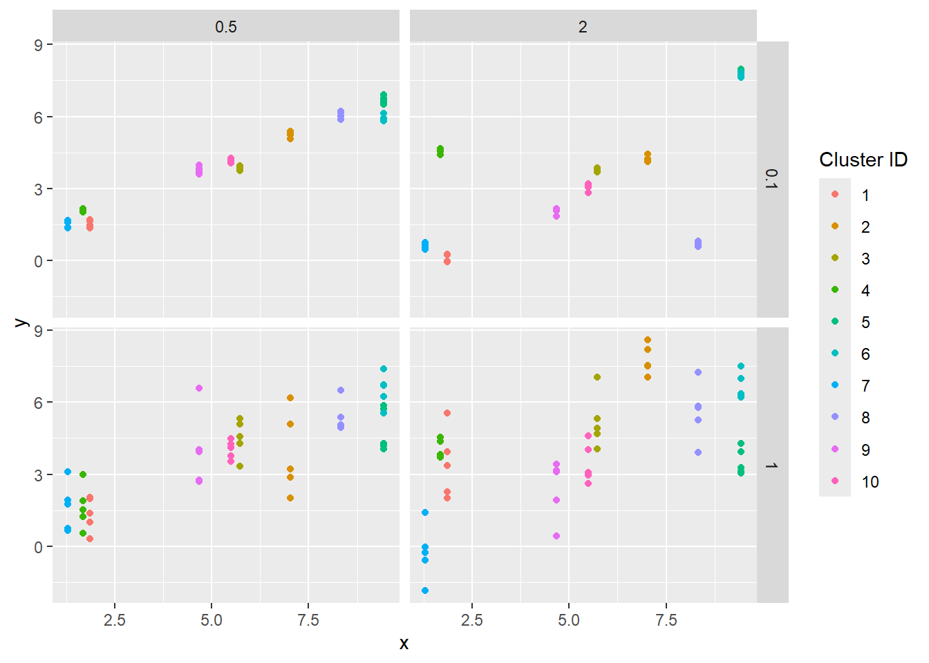
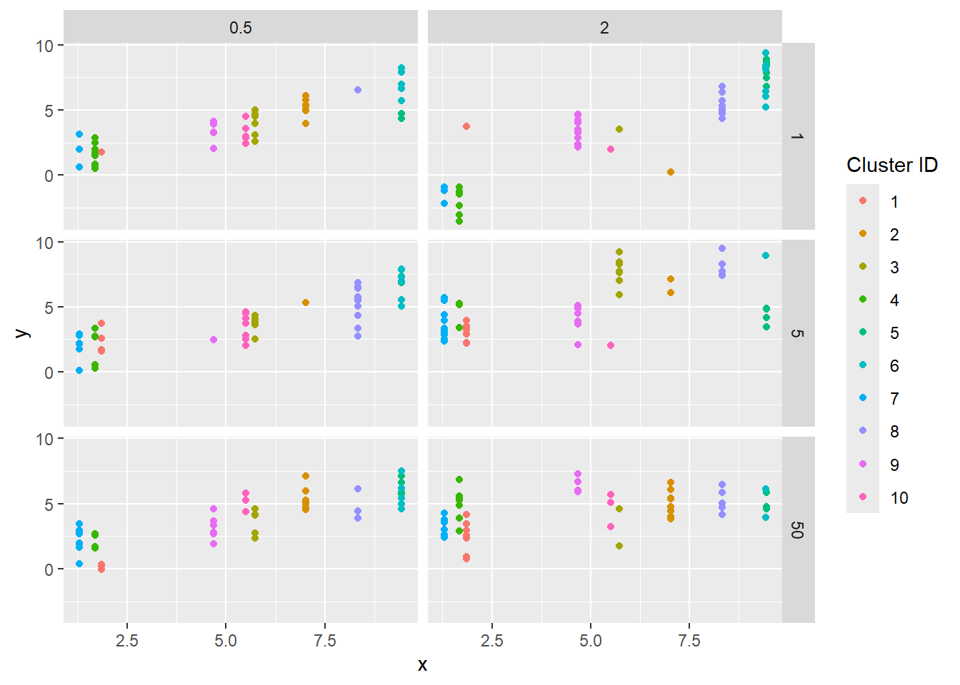
The resulting data; each dot is an observation, the ‘cluster’ (random units) are colors.
sdstacks$points |>ggplot(aes(x = x, y = y, color =factor(cluster, levels =c(1:max(as.numeric(cluster)))))) +geom_point() +facet_grid(obs_sigma ~ sd_rand_intercept) +labs(color ='Cluster ID')
Results
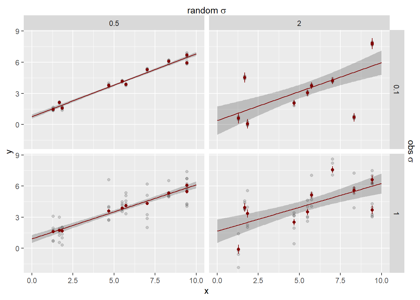
Main result
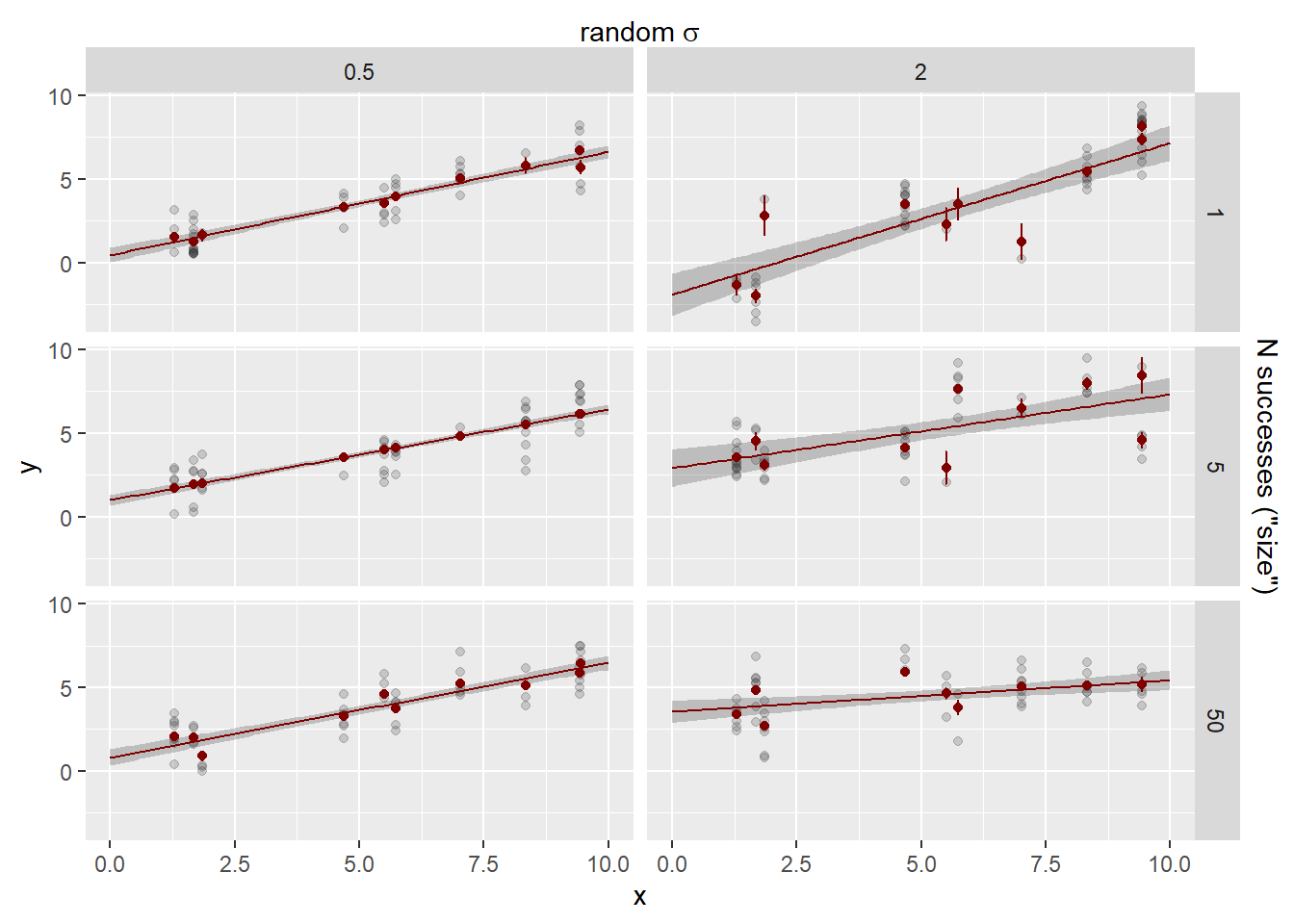
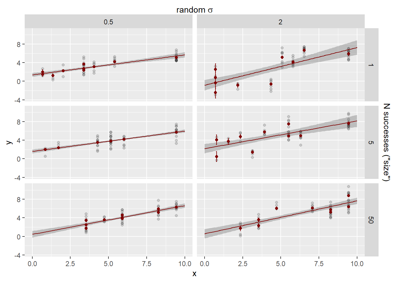
This is the model fit for the full model (line +- se), along with the estimates of the clusters +- se extracted from the full model fit. Gray points are the underlying observations.
sd_fit <-# The estimates +- se out of the model. sdstacks$fitlines |>filter(model =='cluster_rand_x') |>ggplot(aes(x = x, color = model)) +# The raw observationsgeom_point(data = sdstacks$points, aes(y = y), color ='grey20', alpha =0.2) +geom_ribbon(aes(y = estimate, ymin = estimate-se, ymax = estimate + se),alpha =0.25, linetype =0) +geom_line(aes(y = estimate)) +# The cluster estimates with se errorbars out of the modelgeom_point(data = sdstacks$fitclusters |>filter(model =='cluster_rand_x'),aes(y = estimate)) +geom_errorbar(data = sdstacks$fitclusters |>filter(model =='cluster_rand_x'),aes(y = estimate, ymin = estimate-se, ymax = estimate + se)) +scale_color_manual(values = mod_pal) +# facet by random residual sigmas facet_grid(obs_sigma ~ sd_rand_intercept) +scale_x_continuous(sec.axis =sec_axis(~ . , name =TeX(r'(random $\sigma$)'),breaks =NULL, labels =NULL)) +scale_y_continuous(sec.axis =sec_axis(~ . , name =TeX(r'(obs $\sigma$)'),breaks =NULL, labels =NULL))sd_fit +theme(legend.position ='none')
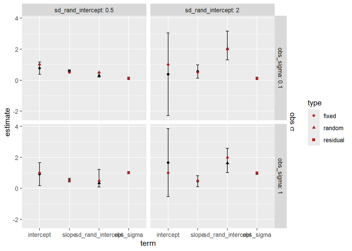
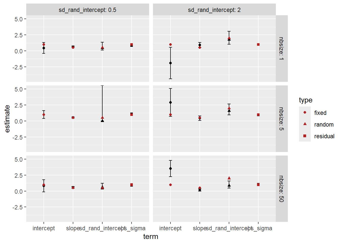
How did we do on the estimates? The error bars here are 95% CI of the estimates. Observation sd does not have an se, it’s the leftovers, and so does not have error bars.
# The plot is nicer than the table# knitr::kable(set_v_est |> # select(-group, `2.5%` = cil, `97.5%` = ciu) |> # mutate(across(where(is.numeric), \(x) round(x, digits = 3))))
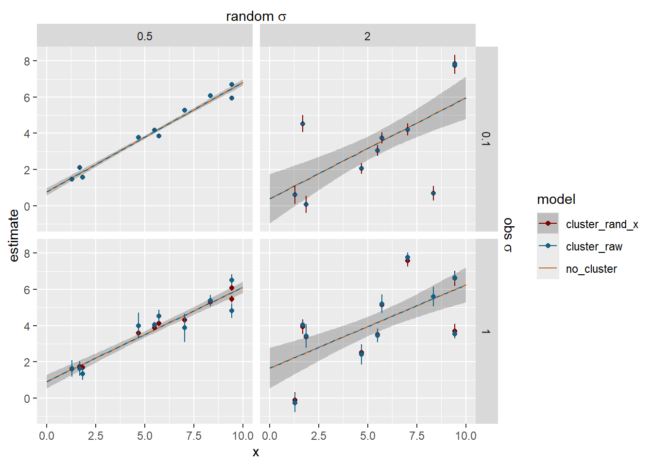
Method comparison
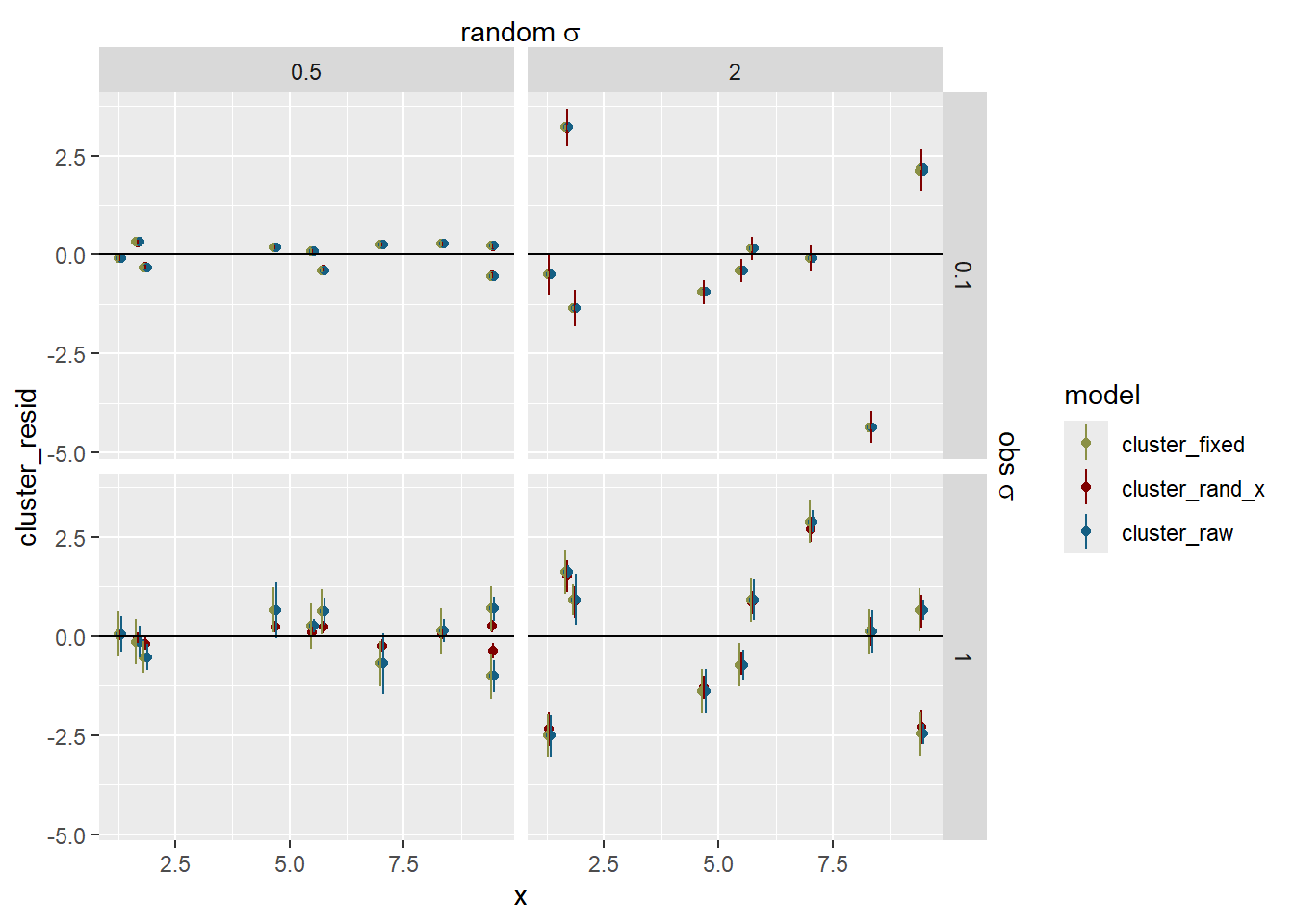
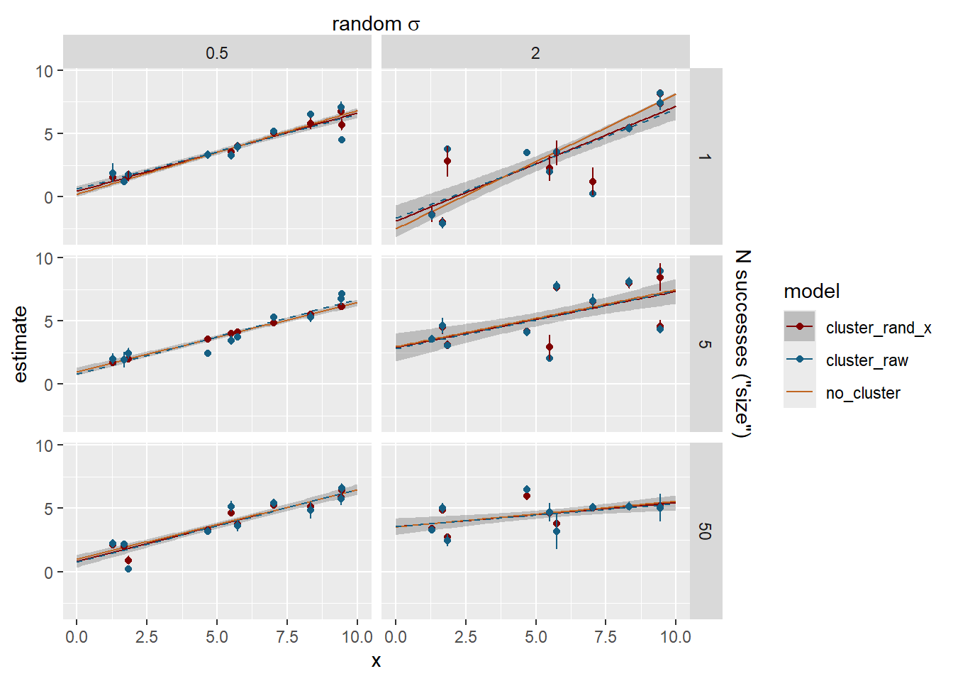
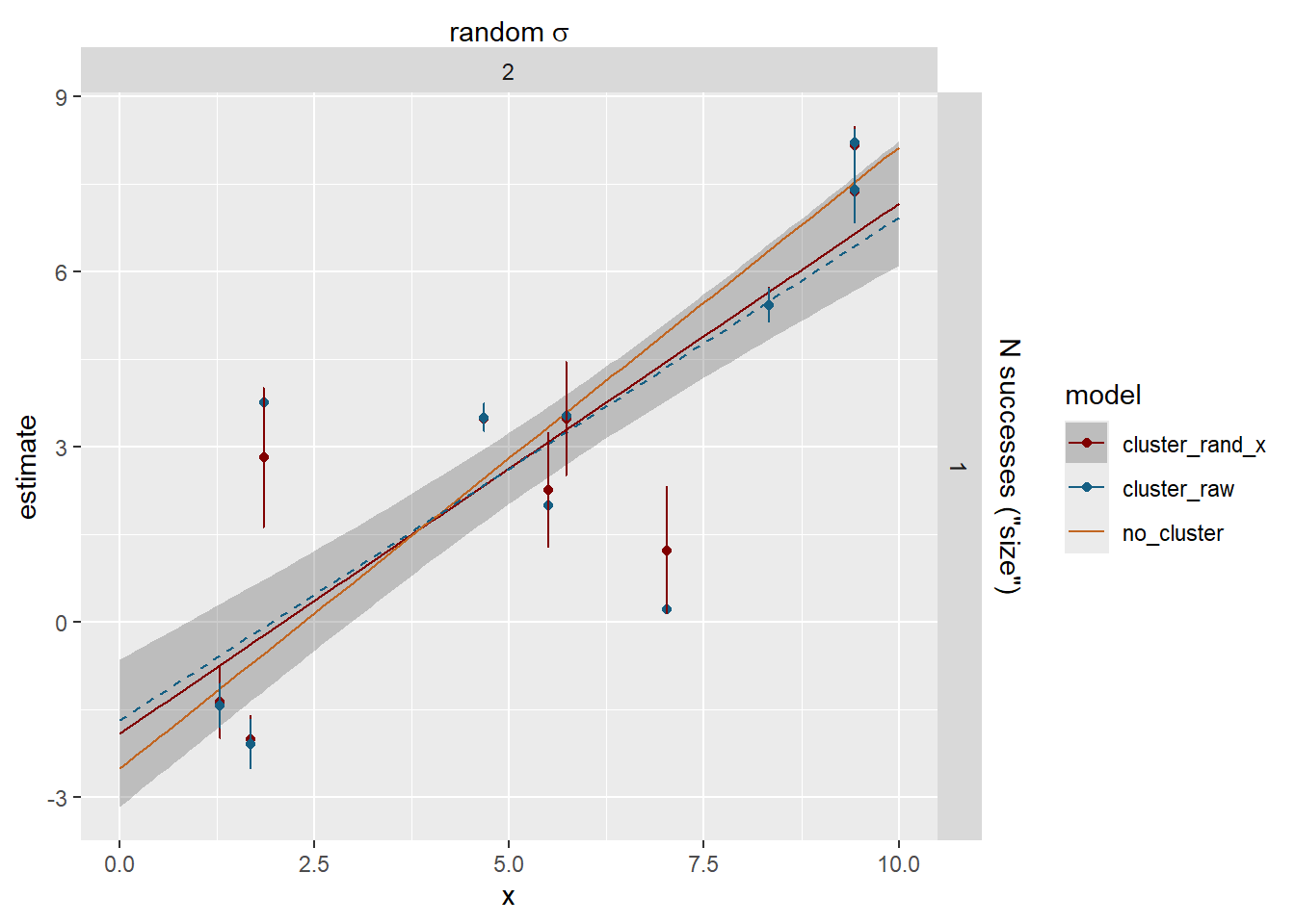
Now, how does that compare with the raw cluster estimates or the fit through the data with no random structure? The dashed blue line is the fit through the raw cluster estimates for visualisation.
Warning: `position_dodge()` requires non-overlapping x intervals.
`position_dodge()` requires non-overlapping x intervals.
`position_dodge()` requires non-overlapping x intervals.
`position_dodge()` requires non-overlapping x intervals.
`position_dodge()` requires non-overlapping x intervals.
`position_dodge()` requires non-overlapping x intervals.
`position_dodge()` requires non-overlapping x intervals.
`position_dodge()` requires non-overlapping x intervals.
Unbalanced groups
For now, we’ll just use two of the options from above, the sd_rand of 0.5 and 2 and sigma of 1, so random variance is half or double residual.
I’m tempted to include an ‘even’ option, but we can either just refer back to the previous or bind_rows the relevant rows.
with_seed(2, unbalparams <-expand_grid(N =50, n_clusters =10,cluster_N ='uneven',nobs_mean ='fixed', # keep simple for nowforce_nclusters =TRUE,force_N =TRUE,# Definitely want 0, the others are essentailly arbitrarynbsize =c(1, 5, 50),intercept =1, slope =0.5,obs_sigma =c(1),sd_rand_intercept =c(0.5, 2),sd_rand_slope =0, rand_si_cor =0,# putting this in a list lets me send in vectors that are all the samecluster_x =list(runif(n_clusters,min =min(xrange), max =max(xrange))),obs_x_sd =0 ))
dropping columns from rank-deficient conditional model: cluster9
dropping columns from rank-deficient conditional model: cluster9
dropping columns from rank-deficient conditional model: cluster9
dropping columns from rank-deficient conditional model: cluster9
dropping columns from rank-deficient conditional model: cluster9
dropping columns from rank-deficient conditional model: cluster9
Joining with `by = join_by(cluster)`
Joining with `by = join_by(cluster)`
Joining with `by = join_by(cluster)`
Joining with `by = join_by(cluster)`
Joining with `by = join_by(cluster)`
Joining with `by = join_by(cluster)`
Joining with `by = join_by(cluster)`
Joining with `by = join_by(cluster)`
Joining with `by = join_by(cluster)`
Joining with `by = join_by(cluster)`
Joining with `by = join_by(cluster)`
Joining with `by = join_by(cluster)`
Warning: There were 6 warnings in `mutate()`.
The first warning was:
ℹ In argument: `fitted_x_lines = map(full_models, function(x) fit_x_full(x,
  xvals = xdata))`.
Caused by warning:
! SE for fits with fixed clusters are not correct
ℹ Run `dplyr::last_dplyr_warnings()` to see the 5 remaining warnings.
Joining with `by = join_by(x, cluster)`
Joining with `by = join_by(x, cluster)`
Joining with `by = join_by(x, cluster)`
Joining with `by = join_by(x, cluster)`
Joining with `by = join_by(x, cluster)`
Joining with `by = join_by(x, cluster)`
Joining with `by = join_by(x, cluster)`
Joining with `by = join_by(x, cluster)`
Joining with `by = join_by(x, cluster)`
Joining with `by = join_by(x, cluster)`
Joining with `by = join_by(x, cluster)`
Joining with `by = join_by(x, cluster)`
Joining with `by = join_by(x, cluster)`
Joining with `by = join_by(x, cluster)`
Joining with `by = join_by(x, cluster)`
Joining with `by = join_by(x, cluster)`
Joining with `by = join_by(x, cluster)`
Joining with `by = join_by(x, cluster)`
# this can be more usefulunbal <-extract_unnest(unbaldata, unbalparams)
Joining with `by = join_by(group)`
Results
Data
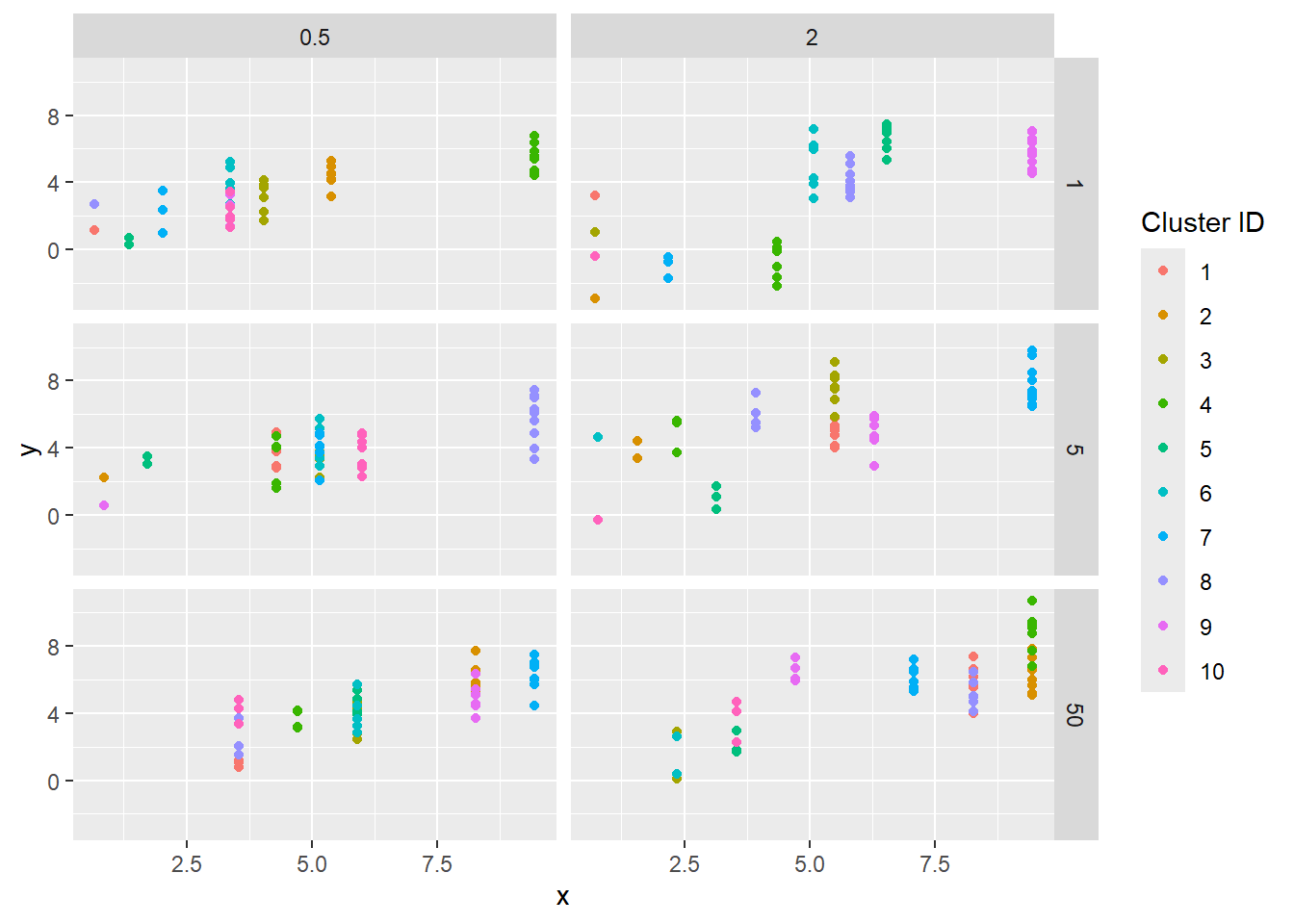
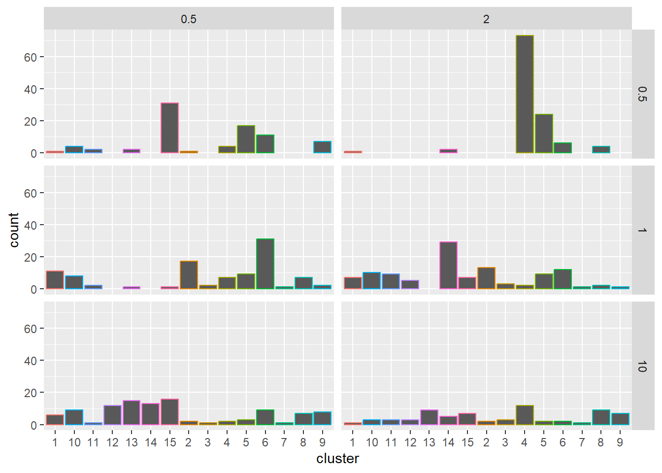
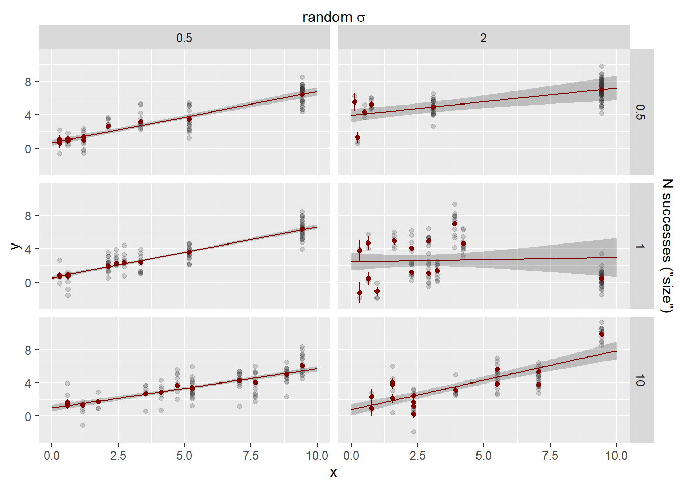
Again, we look at the data, and now can see there are different numbers of points.
unbal$points |>ggplot(aes(x = x, y = y, color =factor(cluster, levels =c(1:max(as.numeric(cluster)))))) +geom_point() +facet_grid(nbsize ~ sd_rand_intercept) +labs(color ='Cluster ID')
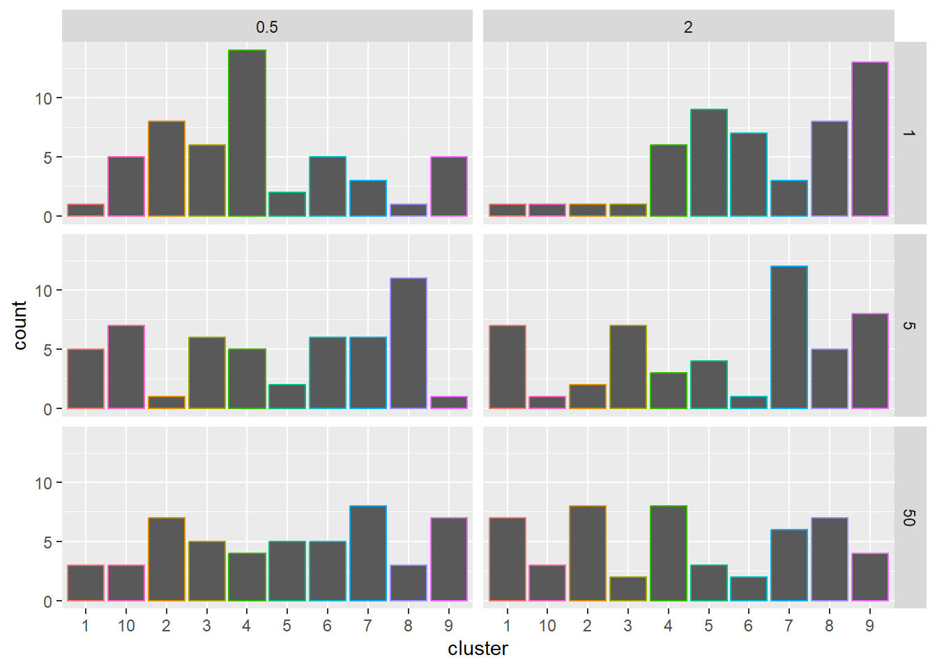
Probably worth being explicit here about the unevenness. I really do think I’m going to want to rethink this to use nbinom. Then once we get to our data, could parameterise based on what we see.
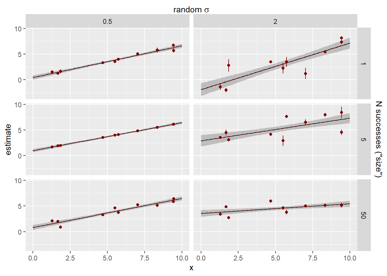
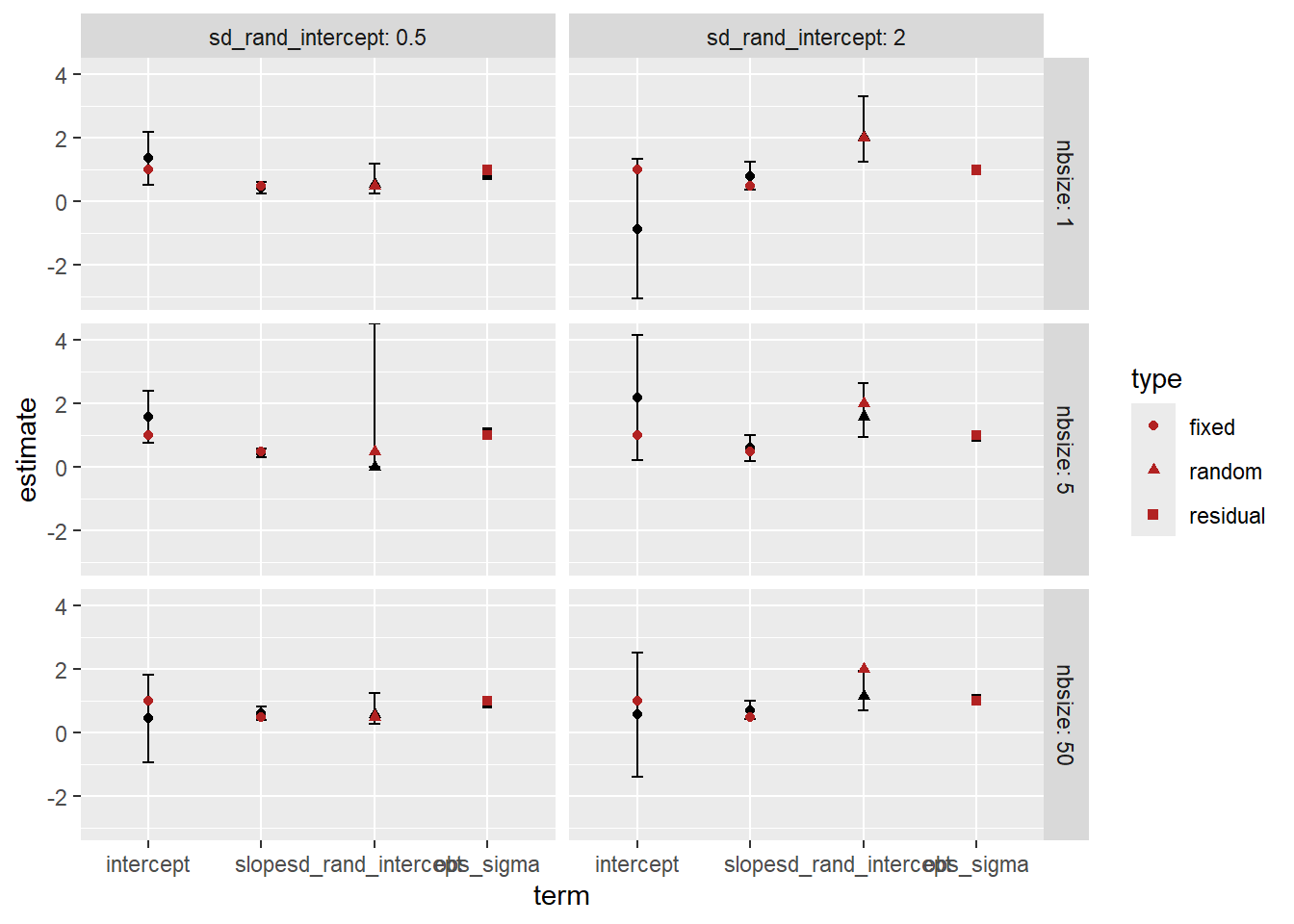
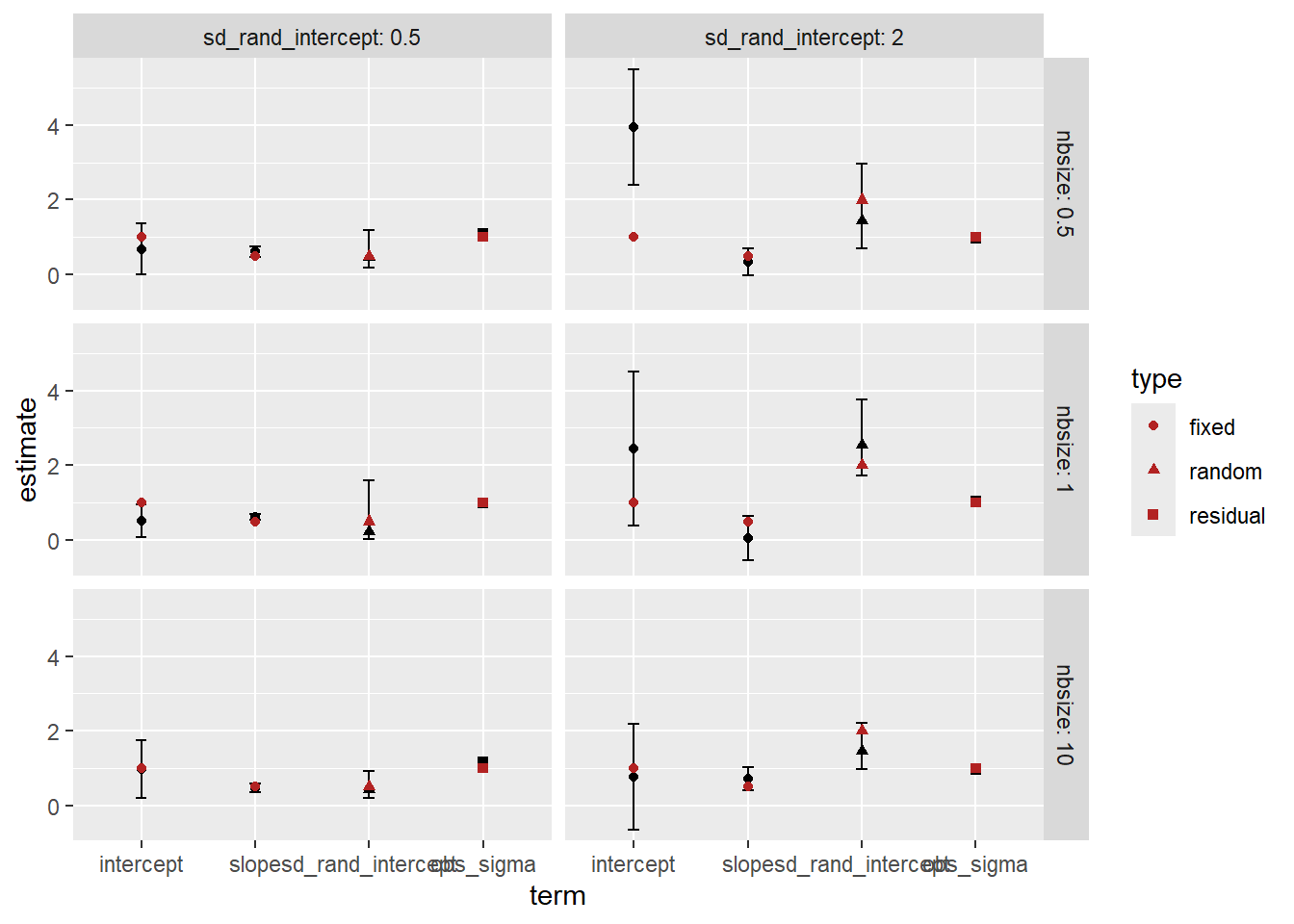
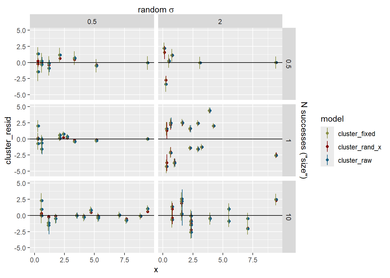
How did we do on the estimates? The error bars here are 95% CI of the estimates. Observation sd does not have an se, it’s the leftovers, and so does not have error bars.
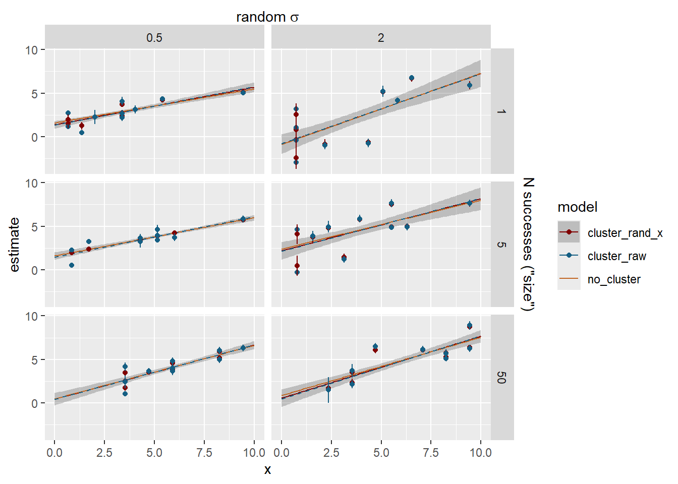
Now we have some meaningful shrinkage and it can cause the lines to deviate. The dashed blue line is the fit through the raw cluster estimates for visualisation.
Warning: `position_dodge()` requires non-overlapping x intervals.
`position_dodge()` requires non-overlapping x intervals.
`position_dodge()` requires non-overlapping x intervals.
`position_dodge()` requires non-overlapping x intervals.
`position_dodge()` requires non-overlapping x intervals.
`position_dodge()` requires non-overlapping x intervals.
`position_dodge()` requires non-overlapping x intervals.
`position_dodge()` requires non-overlapping x intervals.
`position_dodge()` requires non-overlapping x intervals.
`position_dodge()` requires non-overlapping x intervals.
`position_dodge()` requires non-overlapping x intervals.
`position_dodge()` requires non-overlapping x intervals.
Warning: Removed 2 rows containing missing values or values outside the scale range
(`geom_segment()`).
Warning: Removed 4 rows containing missing values or values outside the scale range
(`geom_segment()`).
Warning: Removed 2 rows containing missing values or values outside the scale range
(`geom_segment()`).
Removed 2 rows containing missing values or values outside the scale range
(`geom_segment()`).
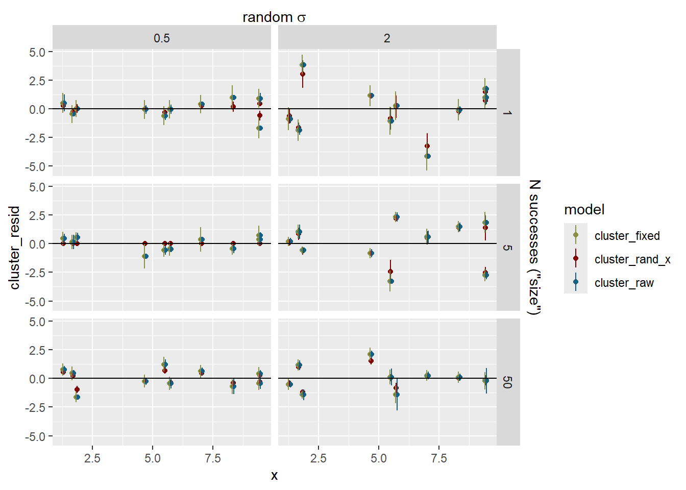
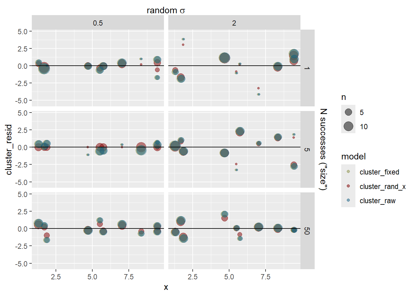
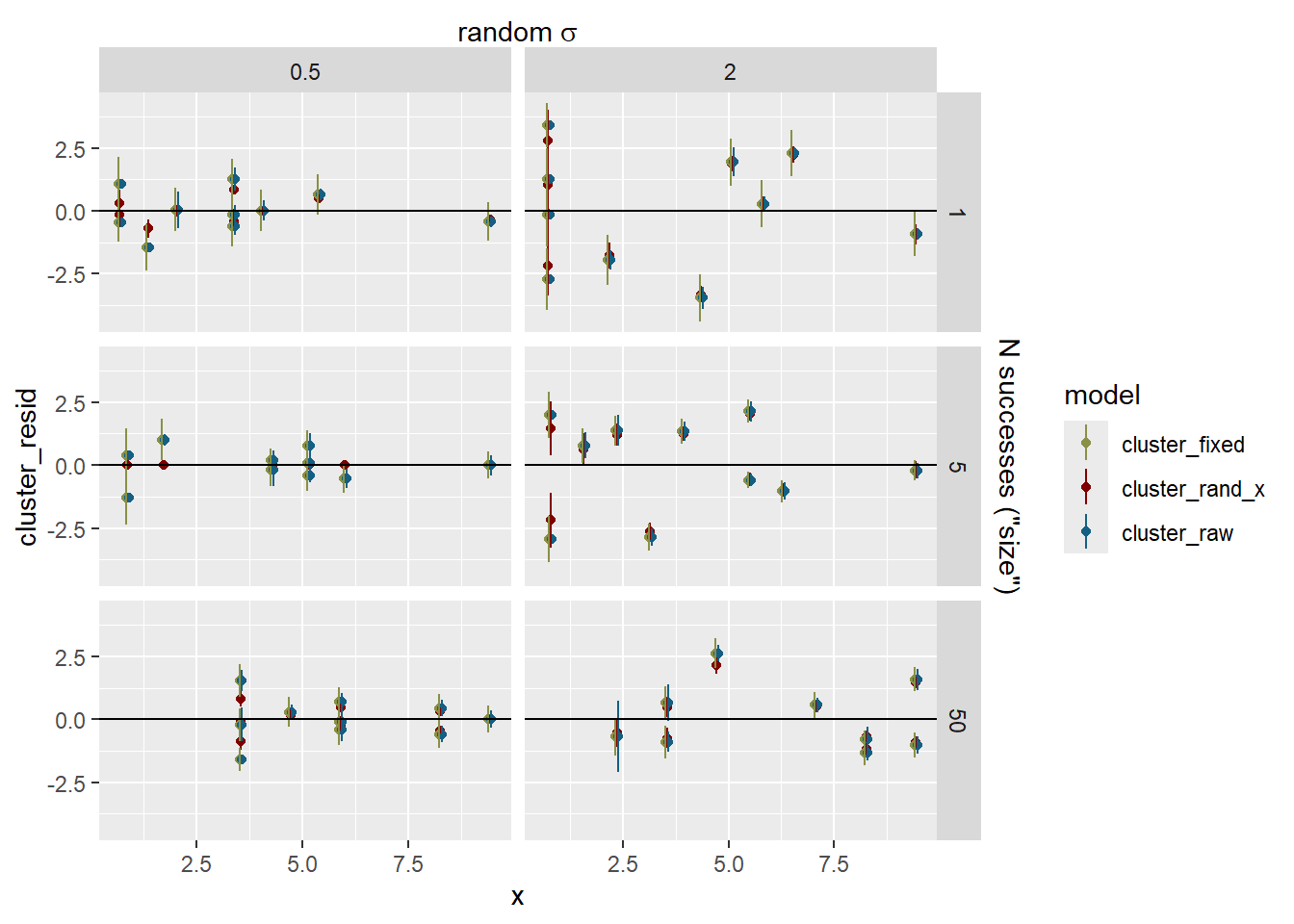
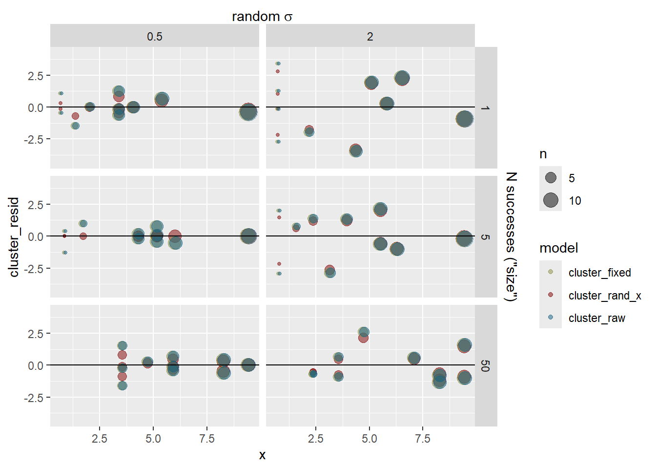
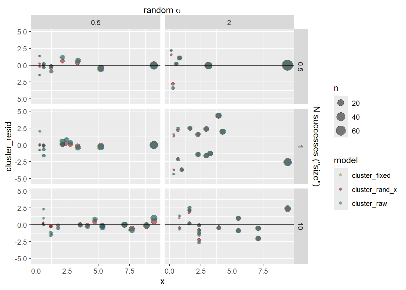
Do the clusters with few observations shrink more? Yes, but not a 1:1 relationship
For now, we’ll just use two of the options from above, the sd_rand of 0.5 and 2 and sigma of 1, so random variance is half or double residual. By using x_is_density = TRUE, we generate the obs among clusters as before, and then calculate density from that. So this should have the same distribution of cluster sizes, but now it’s arranged on x.
with_seed(2, xdensparams <-expand_grid(N =50, n_clusters =10,cluster_N ='uneven',nobs_mean ='fixed', # keep simple for nowforce_nclusters =TRUE,force_N =TRUE,# Definitely want 0, the others are essentailly arbitrarynbsize =c(1, 5, 50),intercept =1, slope =0.5,obs_sigma =c(1),sd_rand_intercept =c(0.5, 2),sd_rand_slope =0, rand_si_cor =0,# putting this in a list lets me send in vectors that are all the samecluster_x =list(runif(n_clusters,min =min(xrange), max =max(xrange))),obs_x_sd =0,x_is_density =TRUE ))
dropping columns from rank-deficient conditional model: cluster9
dropping columns from rank-deficient conditional model: cluster9
dropping columns from rank-deficient conditional model: cluster9
dropping columns from rank-deficient conditional model: cluster9
dropping columns from rank-deficient conditional model: cluster9
dropping columns from rank-deficient conditional model: cluster9
Joining with `by = join_by(cluster)`
Joining with `by = join_by(cluster)`
Joining with `by = join_by(cluster)`
Joining with `by = join_by(cluster)`
Joining with `by = join_by(cluster)`
Joining with `by = join_by(cluster)`
Joining with `by = join_by(cluster)`
Joining with `by = join_by(cluster)`
Joining with `by = join_by(cluster)`
Joining with `by = join_by(cluster)`
Joining with `by = join_by(cluster)`
Joining with `by = join_by(cluster)`
Warning: There were 6 warnings in `mutate()`.
The first warning was:
ℹ In argument: `fitted_x_lines = map(full_models, function(x) fit_x_full(x,
  xvals = xdata))`.
Caused by warning:
! SE for fits with fixed clusters are not correct
ℹ Run `dplyr::last_dplyr_warnings()` to see the 5 remaining warnings.
Joining with `by = join_by(x, cluster)`
Joining with `by = join_by(x, cluster)`
Joining with `by = join_by(x, cluster)`
Joining with `by = join_by(x, cluster)`
Joining with `by = join_by(x, cluster)`
Joining with `by = join_by(x, cluster)`
Joining with `by = join_by(x, cluster)`
Joining with `by = join_by(x, cluster)`
Joining with `by = join_by(x, cluster)`
Joining with `by = join_by(x, cluster)`
Joining with `by = join_by(x, cluster)`
Joining with `by = join_by(x, cluster)`
Joining with `by = join_by(x, cluster)`
Joining with `by = join_by(x, cluster)`
Joining with `by = join_by(x, cluster)`
Joining with `by = join_by(x, cluster)`
Joining with `by = join_by(x, cluster)`
Joining with `by = join_by(x, cluster)`
# this can be more usefulxdens <-extract_unnest(xdensdata, xdensparams)
Joining with `by = join_by(group)`
Results
Data
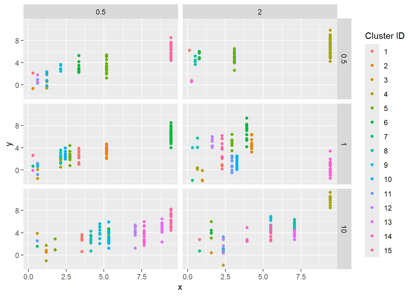
Again, we look at the data, same as above, but now arranged on x.
xdens$points |>ggplot(aes(x = x, y = y, color =factor(cluster, levels =c(1:max(as.numeric(cluster)))))) +geom_point() +facet_grid(nbsize ~ sd_rand_intercept) +labs(color ='Cluster ID')
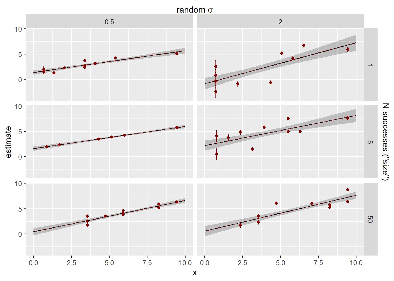
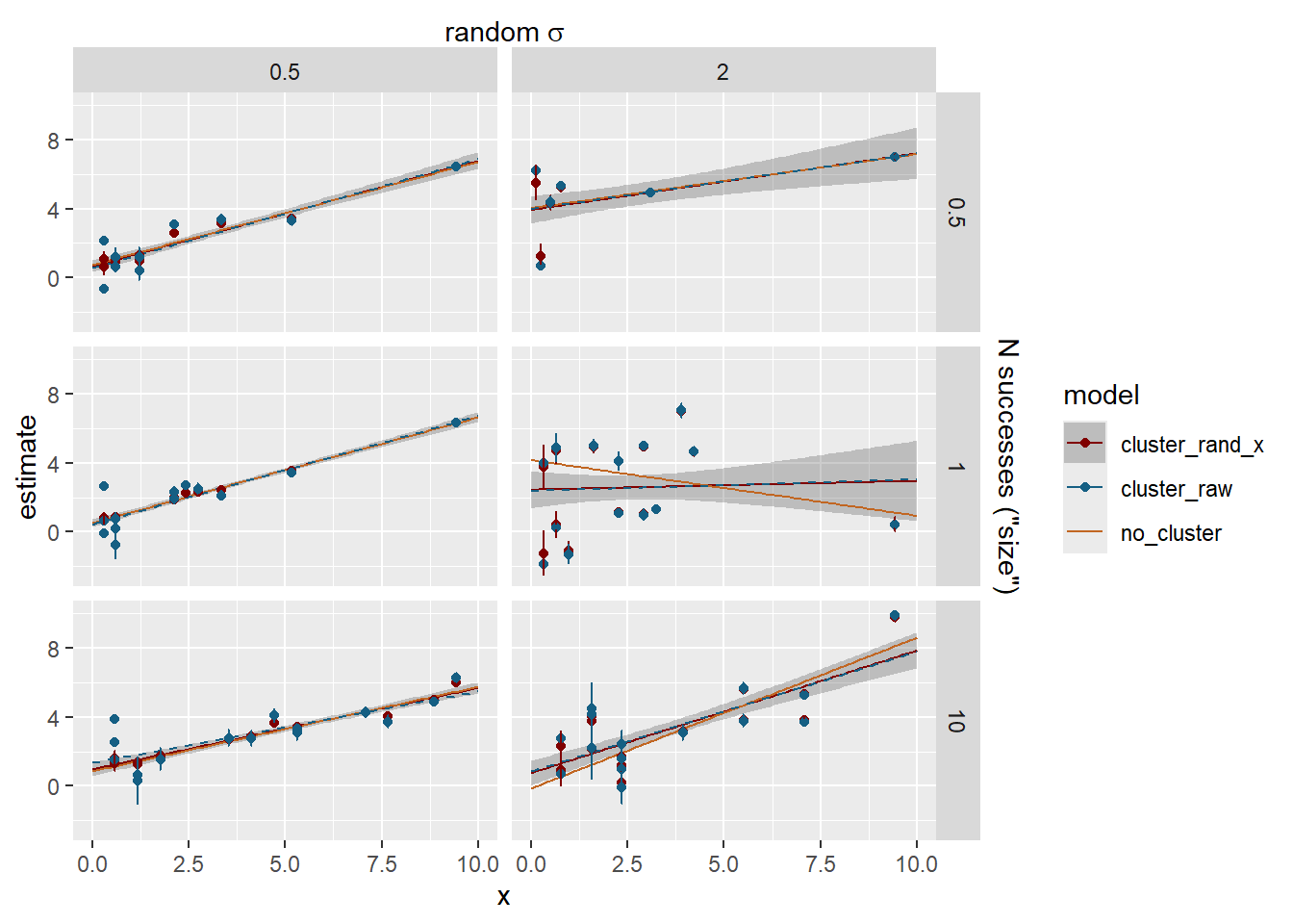
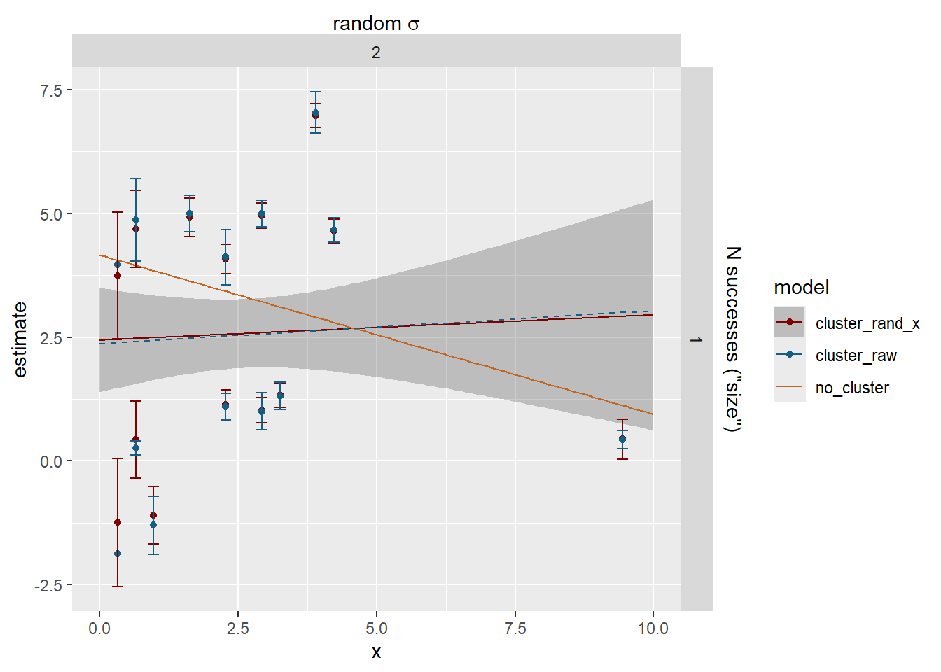
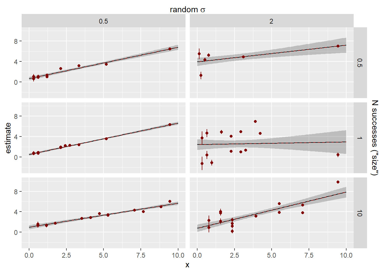
How did we do on the estimates? The error bars here are 95% CI of the estimates. Observation sd does not have an se, it’s the leftovers, and so does not have error bars.
Now we have some meaningful shrinkage and it can cause the lines to deviate. The dashed blue line is the fit through the raw cluster estimates for visualisation.
Warning: Removed 2 rows containing missing values or values outside the scale range
(`geom_segment()`).
Warning: Removed 4 rows containing missing values or values outside the scale range
(`geom_segment()`).
Warning: Removed 2 rows containing missing values or values outside the scale range
(`geom_segment()`).
Removed 2 rows containing missing values or values outside the scale range
(`geom_segment()`).
Do the clusters with few observations shrink more? Yes, but not a 1:1 relationship
So far, there’s not an obvious issue with biased shrinkage. Everything differs from a naive fit without randoms, but that’s clearly wrong anyway.
Larger numbers and freer obs per cluster distribution
I’ll adjust the above to have larger obs and more variance between clusters and also change the nbin mu. Basically crank up the variation and biases. Should I crank up n_clusters? Maybe not (or just a bit), if they’re ‘riffles’.
with_seed(2, bigdensparams <-expand_grid(N =1000, n_clusters =15,cluster_N ='uneven',nobs_mean ='x', force_nclusters =FALSE,force_N =FALSE,# Definitely want 0, the others are essentailly arbitrarynbsize =c(0.5, 1, 10),intercept =1, slope =0.5,obs_sigma =c(1),sd_rand_intercept =c(0.5, 2),sd_rand_slope =0, rand_si_cor =0,# putting this in a list lets me send in vectors that are all the samecluster_x =list(runif(n_clusters,min =min(xrange), max =max(xrange))),obs_x_sd =0,x_is_density =TRUE ))
dropping columns from rank-deficient conditional model: cluster9
dropping columns from rank-deficient conditional model: cluster8
dropping columns from rank-deficient conditional model: cluster9
dropping columns from rank-deficient conditional model: cluster9
dropping columns from rank-deficient conditional model: cluster9
dropping columns from rank-deficient conditional model: cluster9
Joining with `by = join_by(cluster)`
Joining with `by = join_by(cluster)`
Joining with `by = join_by(cluster)`
Joining with `by = join_by(cluster)`
Joining with `by = join_by(cluster)`
Joining with `by = join_by(cluster)`
Joining with `by = join_by(cluster)`
Joining with `by = join_by(cluster)`
Joining with `by = join_by(cluster)`
Joining with `by = join_by(cluster)`
Joining with `by = join_by(cluster)`
Joining with `by = join_by(cluster)`
Warning: There were 6 warnings in `mutate()`.
The first warning was:
ℹ In argument: `fitted_x_lines = map(full_models, function(x) fit_x_full(x,
  xvals = xdata))`.
Caused by warning:
! SE for fits with fixed clusters are not correct
ℹ Run `dplyr::last_dplyr_warnings()` to see the 5 remaining warnings.
Joining with `by = join_by(x, cluster)`
Joining with `by = join_by(x, cluster)`
Joining with `by = join_by(x, cluster)`
Joining with `by = join_by(x, cluster)`
Joining with `by = join_by(x, cluster)`
Joining with `by = join_by(x, cluster)`
Joining with `by = join_by(x, cluster)`
Joining with `by = join_by(x, cluster)`
Joining with `by = join_by(x, cluster)`
Joining with `by = join_by(x, cluster)`
Joining with `by = join_by(x, cluster)`
Joining with `by = join_by(x, cluster)`
Joining with `by = join_by(x, cluster)`
Joining with `by = join_by(x, cluster)`
Joining with `by = join_by(x, cluster)`
Joining with `by = join_by(x, cluster)`
Joining with `by = join_by(x, cluster)`
Joining with `by = join_by(x, cluster)`
# this can be more usefulbigdens <-extract_unnest(bigdensdata,bigdensparams)
Joining with `by = join_by(group)`
Results
Data
Again, we look at the data, same as above.
bigdens$points |>ggplot(aes(x = x, y = y, color =factor(cluster, levels =c(1:max(as.numeric(cluster)))))) +geom_point() +facet_grid(nbsize ~ sd_rand_intercept) +labs(color ='Cluster ID')
How did we do on the estimates? The error bars here are 95% CI of the estimates. Observation sd does not have an se, it’s the leftovers, and so does not have error bars.
Now we have some meaningful shrinkage and it can cause the lines to deviate. The dashed blue line is the fit through the raw cluster estimates for visualisation. Where these are deviating from the no cluster fit, it seems appropriate- they’re equalising the weight between clusters, and not letting the super dense ones pull the whole fit around. Which is right, provided we have enough data to estimate the low ones.
with_seed(2, subparams <-expand_grid(N =10000, n_clusters =10, # 'riffles'n_subclusters =list(c(100, 1000)), # 'rocks' (absolute, not per-riffle I think?)cluster_N ='uneven',nobs_mean ='fixed', # keep simple for nowforce_nclusters =TRUE,force_N =TRUE,# Definitely want 0, the others are essentailly arbitrarynbsize =c(1, 5, 50),intercept =1, slope =0.5,obs_sigma =c(1),sd_rand_intercept =list(c(0.5, 2, 1)),sd_rand_slope =list(c(0, 0, 0)), rand_si_cor =0,# putting this in a list lets me send in vectors that are all the samecluster_x =list(runif(n_clusters,min =min(xrange), max =max(xrange))),obs_x_sd =0 ))
# This is throwing an error, need to fix.subdata <-with_seed(2, make_analysed_tibble(subparams, mod_pal))# this can be more usefulsubout <-extract_unnest(subdata, subparams)
Next
And how does nesting work, especially if it is again uneven?
Explicitly look at singletons? Scaling- if we have 50 singletons at an x, is it as ‘good’ as 1 50?
Then, does the beta introduce additional issues?
AND, finally, what should we plot? What should we DO. It’s one thing to find out the stats are working right and understand why they’re counterintuitive, it’s another to decide how to present them or whether we need to do something else.